Recipe 7. MOPEX/APEX: Point Source Photometry from IRAC Images
This recipe illustrates how to perform point-source photometry from IRAC image data with a relatively uniform background. We show how to use APEX, a photometry package that is part of MOPEX, the MOsaicker and Point source EXtractor. APEX will be used in its multiframe mode, performing detection on coadded data, but point-source fitting photometry on the individual frames. (Aperture photometry is also available, and this is done on the mosaic.) For this example, we will show how you can run all steps in one continuous flow, starting with the Overlap module to correct background levels, and ending with the APEX QA (Quality Assessment) module to examine the quality of the PSF fits. We will demonstrate this using the MOPEX GUI, and we recommend that you also refer to Recipe 4, on using the GUI to mosaic IRAC data. In this recipe, we are analyzing channel 1 (3.6 micron) data from the Galactic First Look Survey (GFLS; http://irsa.ipac.caltech.edu/data/SPITZER/docs/spitzermission/observingprograms/firstlooksurvey/).
Note: With MOPEX release 18.4, default templates will make mosaics with 0.6" pixels, like the PBCD mosaics. This example has been updated to reflect this.
7.1 Requirements
You must have the Spitzer software package MOPEX installed in order to follow along with this recipe (http://irsa.ipac.caltech.edu/data/SPITZER/docs/dataanalysistools/tools/mopex/). This demonstration was originally tested using MOPEX 18.4.9. Use the Spitzer Heritage Archive (http://irsa.ipac.caltech.edu/applications/Spitzer/SHA/) to download the BCD and post-BCD data for AOR 4960000 for this example. See Recipe 1 and Recipe 2 for examples on downloading the data. You will need to request Level 1 (BCD) data and Level 2 + ancillary data (PBCD).
7.2 Have a quick look at your data
It is always a good idea to have a quick look at your data before you proceed with a detailed reduction. The Spitzer pipeline produces a mosaic for just this purpose. To examine it, cd into the Post-BCD area of your data directory:
cd /where/you/unpacked_data/r4960000/ch1/pbcd/
The observations in this particular AOR used the IRAC High Dynamic Range mode for imaging. Hence, there are data for both a short exposure and a long exposure.
Using ds9 or any other viewer of your choice, examine the channel 1 mosaics for the two sets of exposures. The long exposure mosaic is called SPITZER_I1_4960000_0000_8_E8349797_maic.fits, and the short exposure mosaic is called SPITZER_I1_4960000_0000_8_A42451142_maics.fits. (You can find a summary of the IRAC filenaming convention in the IRAC Instrument Handbook.) As you can see, the most recent version of the IRAC pipeline does a pretty good job of producing a mosaic that has a relatively smooth background, etc.
However, you should just about always produce a mosaic yourself, using MOPEX, from the original BCD data. This is not the purpose of this particular recipe, although a science-quality mosaic will be a byproduct of the processing in this recipe.
In the example below, we will be concentrating on point source extraction from the long exposure BCD data. An analogous procedure can be done to perform point source extraction on the short-exposure data, in order to measure the brightnesses of stars that are saturated, or nearly saturated, in the long-exposure data.
7.3 Artifact Mitigation
IRAC BCD data can suffer from several different artifacts, including:
Stray light
Muxstripe
Muxbleed
Column Pulldown
Jailbars
As of version S17.0 of the Spitzer IRAC pipeline, artifact-mitigated images and their associated uncertainty images (*cbcd.fits and *cbunc.fits) are now available in the archive. These images include corrections for column pulldown and banding, induced by bright sources in the images. The corrections are empirical fits to the BCDs and may not always improve the data quality. The standard BCD files (*_bcd.fits) remain available in the archive. The mosaics (pipeline post-BCD products) are now created from the *cbcd.fits images.
In addition to inspecting the post-BCD mosaic, you should also generally inspect the individual CBCD images, to determine whether remaining artifacts can be seen in them and then perform additional artifact mitigation, if necessary.
The data we are considering in this recipe were processed with pipeline version S18.18, as can be seen in the file
so, some artifact mitigation has already been performed. For this reason, we will use the *cbcd.fits files. We will also assume the corrections were good, and use the original uncertainty files, *bunc.fits.
7.4 Set up files in preparation to run MOPEX
Before we can run MOPEX to compute the overlap correction, mosaic the data, and perform point source extraction, we need to do a little preparation.
Make a list of the CBCD (*cbcd.fits), uncertainty (*bunc.fits), and bad pixel mask (*bimsk.fits) files in the directory /where/you/unpacked_data/. For this recipe, the lists should include only the odd-numbered frames, which have long exposure times (header keyword HDRFRAME = long). For your convenience, we provide a shortened list of image files for the demonstration here:
Remember to edit these files so that each line contains the full paths to the data on your computer.
We can run each of the steps below in sequence, or we can load each of the individual pipelines into a flow in MOPEX and run the flow all the way through. We choose to do the latter here. However, you could certainly run as a flow each pipeline separately, adding a new pipeline after running a previous one.
7.5 Compute the overlap correction
First, we must match the backgrounds in overlapping IRAC frames. The Overlap Pipeline in MOPEX does this by calculating an additive correction for each CBCD image, to bring them to a common background level. Follow these steps to run the overlap pipeline on the corrected BCDs. But do not run the flow yet -- that will come later.
1. Start up the MOPEX GUI.
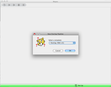
2. Under the File menu, select a New Overlap Pipeline. Click on "File"-->"New Overlap Pipeline..."-->"Overlap, IRAC ch1"-->click "OK".
You will see the previously empty MOPEX window fill up with the Overlap flow.
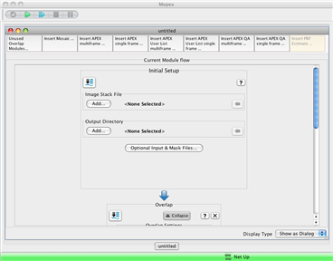
3. Set parameters in MOPEX Overlap Flow.
Below is the minimum set of parameters that should be set in running overlap. A full description of each of the parameters is provided in the MOPEX User's Guide and is also discussed in the IRAC COSMOS Recipe (Recipe 3).
a. Image Stack File should be the gfls_cbcd.txt file you downloaded and edited previously.
b. Output Directory is a directory you create, e.g., /where/you/unpacked_data/ch1/bcd/output/.
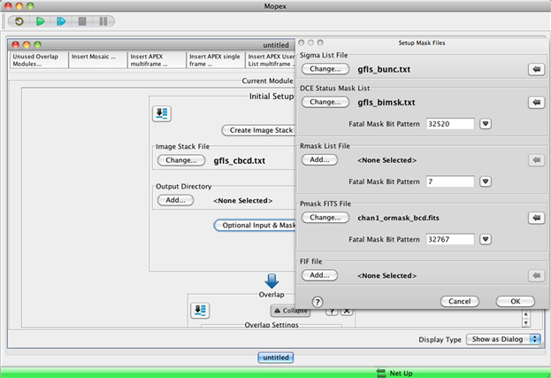
c. Optional Input & Mask Files -- Sigma List File should be the gfls_bunc.txt file you downloaded and edited previously.
d. Optional Input & Mask Files -- DCE Status Mask List should be the gfls_bimsk.txt file you downloaded and edited previously.
e. Pmask FITS file � The GUI template will load a default Pmask (permanent bad pixel mask) file that should be good for most purposes. Date-specific Pmasks for IRAC are available in the cal/ subdirectory where you installed MOPEX, e.g., /your_home_directory/mopex/cal/ (assuming MOPEX is installed in your home directory). You can check that you have the latest versions as follows. A tarball of the Pmasks can be found at http://irsa.ipac.caltech.edu/data/SPITZER/docs/irac/calibrationfiles/pmask/. You can unpack the tarball in cal/. (This will overwrite any potentially older versions of these files.) To decide which Pmask to use, look at the date your BCDs were observed. From the keyword DATE_OBS in the fits header of the BCD files, we find that these data were taken on December 6, 2003. Look in the cal/ subdirectory for the Pmasks closest in time to the observation date; in this case, those in the mar04/ subdirectory. To verify that the channel 1 Pmask file here, i.e., the file /your_home_directory/mopex/cal/mar04/mar04_ch1_bcd_pmask.fits is the appropriate one, you can look at its header for the keywords STRTDATE and ENDDATE to see the date range for which the Pmask is applicable. Since this date range is August 1, 2003 to May 2, 2004, we see that this is the right one.
We could make a quick mosaic within Overlap to see how good the corrections were. But we will skip that step and make a better mosaic by inserting a Mosaic step. It will use the overlap-corrected frames automatically.
7.6 Produce a Science Mosaic
Now that we have corrected the BCDs for mismatched backgrounds, the next step is to use the corrected BCDs to produce a new mosaic.
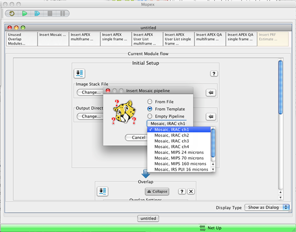
1. Insert a Mosaic Pipeline into the flow.
On the MOPEX GUI, click where it says, "Insert Mosaic ...." In the dialog box, select "From Template," and "Mosaic, IRAC ch1," and click "OK."
By-and-large, the default parameters for this pipeline can be used. As described in the "Basic Concepts: Outlier Detection" section of the online MOPEX manual, MOPEX has four algorithms for identifying bad pixels: single-frame, multiframe temporal, dual outlier, and box outlier. The single-frame outlier method is not normally needed. For low coverage data like ours (the AOR we have chosen has a coverage ~4), you should use either dual outlier or box outlier, or both. The default IRAC Mosaic template uses all three main methods. Since dual and box are both present, we can leave this as it is.
Additionally, as described in the MOPEX User's Guide, four interpolation schemes are implemented: Default, Drizzle, Grid and Cubic. General guidelines for choosing the interpolation scheme appropriate for your data set are provided in the Helpdesk knowledgebase: "How do I decide which interpolation method in MOPEX to use to create my science mosaic?". A rule of thumb is that if you have a coverage of 10 or less (as we do), you will probably want to use the default interpolation scheme.
If you have higher coverage data than the low coverage data we are analyzing here, you may wish to use a different outlier rejection scheme and a different interpolation method. For a medium-deep coverage example, see the IRAC COSMOS recipe (Recipe 3).
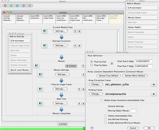
As discussed in the IRAC Instrument Handbook (http://irsa.ipac.caltech.edu/data/SPITZER/docs/irac/iracinstrumenthandbook/), the IRAC flat-field is derived by imaging the high surface brightness zodiacal background, and the spectrum of the zodiacal background peaks redward of the IRAC filters. However, the spectral energy distribution of many sources, particularly stars, have color temperatures that peak blueward of the IRAC filters. A variation also exists in the effective filter bandpass of IRAC as a function of angle of incidence, which in turn depends on the exact position of an object on the array. Photometry of blue sources like stars needs a correction factor. There are two ways to do this. The first, more exact, method is to correct the (C)BCD frames before making the mosaic. The second, approximate, method is to create a mosaic of correction factors, and multiply extracted fluxes by the value in the correction mosaic at the same position as the object. The GUI is currently set up to create the correction mosaic for the second method.
You can make the correction mosaic easily within the Mosaic pipeline using the GUI, by clicking on the "Settings" button in the Mosaic Settings module of the pipeline. In the resulting dialog box, if you click on "Spitzer Cryo Default," under "Array Location Dependent Photometric Correction Mosaic," the appropriate files that you need to apply this correction (in this case, ch1_photcorr_rj.fits and ch1relpixarea.fits) will be input. These files can be found in cal/. Then from the Add to Mosaic window click on "Make Array Correction Files" and "Make Array Correction Mosaic" to add these to the flow. The correction mosaic will go into the same output directory as the normal mosaic. Refer to Recipe 6 for more detailed instructions on how to build an array location dependent mosaic.
7.7 Perform APEX Multiframe photometry
As part of this flow, we are constructing a science-grade mosaic. But for IRAC, point-source fitting needs to be done on the individual (C)BCD frames, not on the mosaic. (Aperture photometry will be done on the mosaic.) For the point-source fitting, we will use a map of the spatially-variable PRF for the highest accuracy.
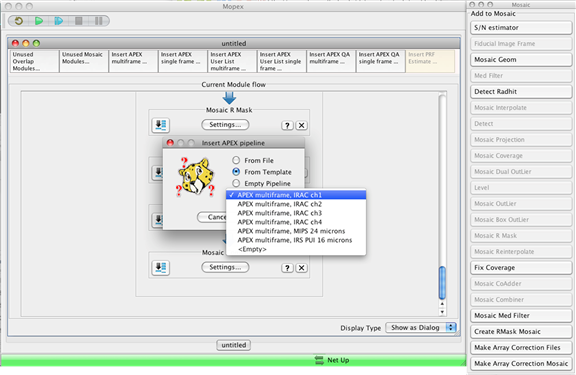
1. Insert APEX Multiframe pipeline
On the MOPEX GUI, click where it says, "Insert APEX multiframe...." In the dialog box, select "From Template," and "APEX multiframe, IRAC ch1," and click "OK."
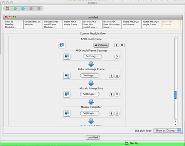
You will see the APEX Multiframe pipeline inserted into the overall flow.
2. Point APEX Multiframe to a PRF Map
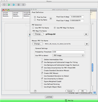
The MOPEX GUI by default has the PRF selection, under the APEX Multiframe settings dialog, as the file apex_sh_IRAC1_col129_row129_x100.fits, which is located in the /your_home_directory/mopex/cal/ subdirectory. Although you can run APEX with just this PRF, relevant to the IRAC frame pixel center, we recommend using the whole set of PRFs, in a PRF Map, as this noticeably improves the quality of the PRF fitting for sources outside of the central region of the arrays. The set of PRFs for channel 1 can be found at http://irsa.ipac.caltech.edu/data/SPITZER/docs/irac/calibrationfiles/psfprf/070131_prfs_for_apex_v080827_ch1.tar.gz and the corresponding PRF Map file can be found at http://irsa.ipac.caltech.edu/data/SPITZER/docs/irac/calibrationfiles/psfprf/prfmap.tbl. The gzipped tarball of PRF FITS files can be unpacked in the /your_home_directory/mopex/cal/ subdirectory. Edit the prfmap.tbl file so that the prf file names contain the full directory path. For example, the line for PRF_Filename_1 might look like:
In APEX Multiframe Settings, select "Use PRF Map File Name" and choose prfmap.tbl. In "Mosaic PRF File Name" ensure the following file from the cal/ directory is present: IRAC1_06_mosaic_4x_detect_kernel.fits. In the default template, APEX needs this to detect on the 0.6" pixel mosaic.
The rest of the default settings should be acceptable for the present purposes. But the default settings for APEX will create a crude mosaic (no outlier rejection). Since we already are creating a mosaic, we need to remove some modules from the APEX flow.
Simply click on the "X" to the far right in the modules, "Fiducial Image Frame," "Mosaic Interpolate", "Mosaic CoAdder," and "Mosaic Combiner." This will remove these modules from the flow.
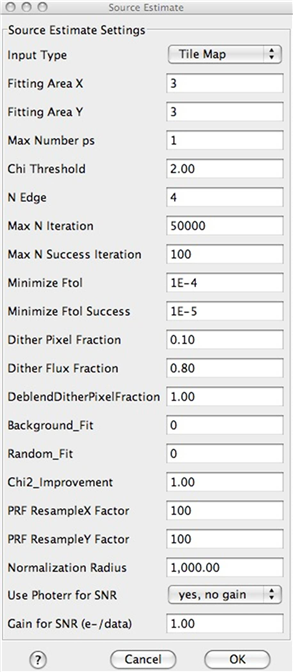
3. Check the Source Estimate Settings
Most, if not all, of the default settings for the Source Estimate module are fine to use without modification. Check these settings by clicking on "Settings" in the module window. In particular, if you are performing PRF fitting with the "100×"-sampled PRFs, either the single, center-frame PRF or the PRF Map (recommended), you should be sure that the "Normalization Radius" is set to the value "1,000.00." (The "standard aperture" for the IRAC absolute calibration is 10 pixels; these model PRFs have been 100-times-sampled, hence, 10 pixels × 100 = 1,000 pixels.) This will ensure that the PRF flux normalization is matched to the IRAC calibration standard radius.
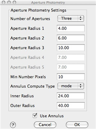
5. Examine the Settings in the Aperture Photometry module.
Click on the Settings button in the Aperture Photometry module. Note the default aperture radii of 4.0, 6.0, 10.0 in 0.6" mosaic pixels correspond to BCD image apertures (2.0, 3.0, 5.0 BCD pixels) for which aperture corrections are available in the IRAC Instrument Handbook. A choice of 20.0 (10.0), together with the annulus settings of Inner Radius of 24 (12) and Outer Radius of 40 (20), would correspond to the standard aperture used for IRAC flux calibration. If desired, add this aperture. However for typical sources in typical fields, this is too large of an aperture for science purposes.
7.8 Perform Quality Assessment of the PRF Fitting
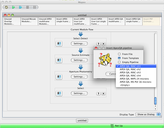
1. Insert the APEX QA Multiframe pipeline
To assess the quality of the PRF fitting on the BCD frames performed in the APEX Multiframe pipeline, we can use the APEX QA Multiframe pipeline. This module can subtract fitted PSFs from the BCD frames and optionally mosaic those residual frames. It will reveal if some sources have been over- or under-subtracted, e.g. due to difficulty fitting a close blend of sources.
Above the flow, click on the box "Insert APEX QA multiframe...". In the dialog box, select "From Template" and "APEX QA, IRAC ch1" and click "OK".
If desired, click on the Apex QA Settings. You will see it is expecting an Extract table: a list of positions and fluxes to subtract. Click "Cancel". The GUI will recognize that Apex is in the flow, and it will get the Extract table, FIF, and PRF from that run.
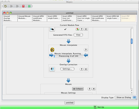
7.9 Run the Flow
You are now ready to run the complete flow, end-to-end, from input (C)BCDs to the mosaic of image residuals! Click the large, green "arrow" button toward the top-left corner of the MOPEX GUI, and the flow will get underway. A query box will come up at the end asking whether you want to delete intermediate files. This is usually acceptable.
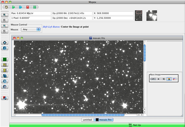
When the flow is completed, we can examine some of the output. Scroll back to the bottom of the Mosaic pipeline, to the Mosaic Combiner module, and click on "Mosaic image file". The mosaic you made (<output>/Combine-mosaic/mosaic.fits) is shown in the image window.
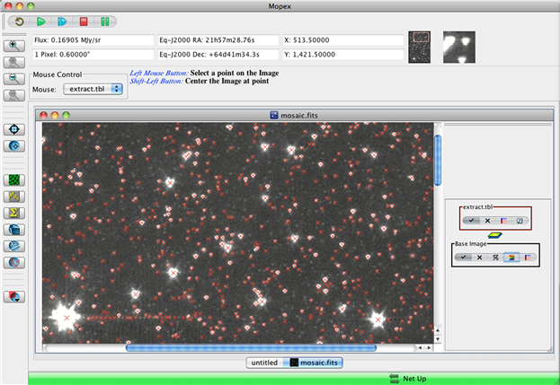
There are two ways to overlay the final extract table on the mosaic. The first is a general Overlay tool. Go up to Overlays in the top MOPEX menu bar, select "Catalog File" and choose <output>/extract.tbl. The sources will be overlaid on the mosaic. (An additional table file, extract_raw.tbl, contains the raw extractions before the Select module in APEX was run.) The second way is to scroll to the APEX flow, Select window, and click "Overlay Output Table on mosaic.fits.
As you can see, APEX with its default parameters did a good job of detecting point sources in the regions away from the bright objects. Around bright objects (or in complex backgrounds) it can sometimes have difficulty identifying true sources. So it is worth examining the results carefully in these regions. In the worst cases, you can input your own "Detect" list to the point-source photometry steps using the APEX User List module. Unfortunately, APEX also detected "sources" which are clearly artifacts created by the brighter sources (lower left of image above). These artifacts are the result of muxbleed, which is not completely corrected in the version of the IRAC pipeline used to process these images. An IRAC artifact mitigation code, written in IDL, can be used to correct for muxbleed, after first correcting for source saturation (the routine "Iracworks," to perform saturation correction, can also be found at that site). For this recipe, we clearly did not run this artifact mitigation code. We recommend that you perform artifact mitigation on your IRAC (C)BCD data before running this flow and performing photometry.
We can check how well the PRFs fit the point sources. At the bottom of the APEX QA flow in the Mosaic Combine window, select "Mosaic Residual Images - Image File". This will display the residual mosaic (<output>/Residual/mosaic/Combine/mosaic.fits).
Finally, the fluxes in the extract.tbl file require two types of small corrections for the highest accuracy. The point-source fitted fluxes are in the column "flux" and the best uncertainty estimate is given as a signal-to-noise ratio in the column "SNR". Because of differences in normalization between IRAC data and APEX, a small correction needs to be applied to "flux". These are given in Appendix C.3, Table C.1 of the IRAC Instrument Handbook. For example, for IRAC1 divide "flux" by 1.021. For bright, isolated point sources, this correction should give photometry whose median is within about 2 % of standard aperture photometry.
The second correction is the array-position dependent color correction discussed above, and applies to both point-source fitting and aperture photometry (e.g. columns "aperture2" and "ap_unc2"). Use the correction mosaic you made in <output>/Combine-mosaic/mosaic_arraycorr.fits to correct photometry. (There is no MOPEX GUI tool for this at present.) Multiply final point-source fitted or aperture fluxes by the correction factor at the source position for blue (star-like) sources. The correction factor goes to 1 for red sources, where red is like the zodiacal emission. Corrections for intermediate colors can be found by interpolation.
You should now generally be able to apply this recipe to other IRAC channels and other science cases with relatively uniform backgrounds.