Recipe 9. Spitzer Synthetic Photometry
If you have a template source spectrum, you may wish to predict the calibrated flux densities that would be reported in the various Spitzer bands (e.g. IRAC 3.6, 4.5, 5.8, 8.0 microns; IRS Peakup Imaging 16, 22 microns; MIPS 24, 70, 160 microns). This can be useful, for instance, in deriving photometric redshifts. After introducing the relevant basic concepts, this section provides step-by-step instructions for determining synthetic, calibrated IRAC, IRS, and MIPS photometry from such a template.
9.1 Requirements
In this section we have collected information which will be useful to those who wish to compute synthetic Spitzer photometry. We also provide IDL code (only tested on IDL version 6.3) which can calculate synthetic fluxes for smooth spectra (generally not pure emission lines). Examples using the code are provided. The IDL code is available on the SSC web site here: http://irsa.ipac.caltech.edu/data/SPITZER/docs/dataanalysistools/cookbook/files/spitzer_synthphot_28Oct2008.tar.gz.
Unpack the gzipped tar file in a directory that is included in your IDL path:
gunzip spitzer_synthphot_28Oct2008.tar.gz
tar xvf spitzer_synthphot_28Oct2008.tar
Among the files you just unpacked are the filter response files (ending in .txt and .dat). These are assumed to be in your working directory in the following examples.
Note that this IDL code provides good agreement with the values tabulated in the IRAC, MIPS and IRS Instrument Handbooks. The results are consistent to within half a percent. The fact that the values are not exactly the same is likely due to differences in the interpolation and integration methods used. The differences in color correction are comparable to the errors in the measurement of the spectral response curves and will be less than the systematic error due to real differences between the assumed spectral shape and the observed object.
Note that this IDL code computes color corrections for the IRS peak-up filters as calibrated in pipeline versions S17 and greater. It is not to be used for data reduced with older versions of the pipeline.
9.2 The Basics
9.2.1 Useful Definitions
There are three quantities that are essential for understanding how to perform synthetic photometry for the Spitzer instruments on a given template spectrum.
- λeff: This is the effective wavelength of the filter. These are defined and tabulated for each Spitzer instrument in the step-by-step guides below.
- ƒn(λeff): This is the monochromatic (measured at the effective wavelength of the filter) flux density of the template spectrum.
- ƒnSpitzer: This is the calibrated Spitzer flux density that would be reported (by e.g. MOPEX/APEX) if the template spectrum were observed by one of Spitzer's imagers. It corresponds to the monochromatic (measured at the effective wavelength of the filter) flux density of a source that
- has a standard spectral shape (defined independently for each filter; see the step-by-step guides below); and
- results in the same observed counts as the template source.
Thus, ƒνSpitzer = ƒν(λeff) if the template spectrum has the standard spectral shape. However, significant deviations can occur if the template, or source, spectrum is very different than the standard, or reference, spectrum.
- K: This is the color correction, which relates the above two quantities according to:
 . The color correction is computed in a different way for each of Spitzer's imagers (see the step-by-step guides below). It requires knowledge of 1) the source spectrum, 2) the reference spectrum, and 3) the filter response.
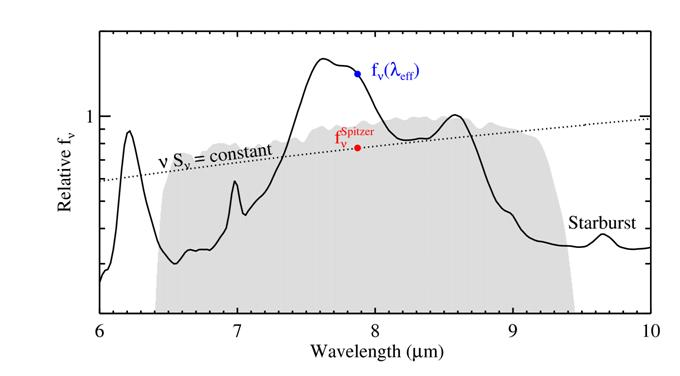
The plot below illustrates these concepts. For this example, we use the average starburst spectrum (http://www.strw.leidenuniv.nl/~brandl/SB_template.html) from Brandl et al. 2006 (http://adsabs.harvard.edu/abs/2006ApJ...653.1129B). We wish to determine the calibrated IRAC flux density that would be reported if this template source were observed in channel 4 (8 microns). The grey shaded region shows the arbitarily-normalized response function for the IRAC channel 4 filter, in units of electrons per photon. The blue point shows ƒν(λeff), which is simply the value of the template spectrum at the effective wavelength. However, since a starburst galaxy has a very different shape than the reference spectral shape for IRAC (νSν = constant), ƒνSpitzer is significantly different from ƒν(λeff). To figure out how different, we must find the constant that will make the total counts from a νSν = constant spectrum the same as that from the starburst galaxy. The appropriately-normalized flat spectrum is shown as a dotted line in the figure below. To find ƒνSpitzer, we simply evaluate this normalized flat spectrum at the effective wavelength. The result is shown as a red point. The ratio of these two quantities is just the color correction, which in this case is 
The IDL code used to create the above graph is available on the Spitzer web site here: http://irsa.ipac.caltech.edu/data/SPITZER/docs/dataanalysistools/cookbook/files/spitzer_synthphot_example.pro.
9.2.2 Differences between IRAC, IRS, and MIPS photometry
The background information provided above applies to all Spitzer photometry from the IRAC, IRS, and MIPS instruments. However, the details are different for each instrument. The two main differences are:
- The filter response curves are given in units of electrons per unit energy for MIPS and in units of electrons per photon for IRAC and IRS. Therefore, the equation used to calculate the color correction from the provided response function is different for MIPS than for IRAC and IRS. These differences are outlined in the step-by-step procedures provided below for each instrument.
- The reference spectrum has the shape of a 10,000K blackbody for MIPS and that of a flat spectrum (nSν = constant) for IRAC and IRS.
9.2.3 Converting from Spitzer photometry to other systems
In modern astronomical literature there are several reference systems in common use (SI, CGS, Jy, AB, Vega, etc). Each of these systems adopts a different reference spectrum. We have noted above that the IRAC and IRS systems adopt a reference spectrum described by νSν = constant, while the MIPS system is based on a 10,000 Kelvin blackbody. In constrast, the AB and Jansky systems assume νSν = constant, while the Vega system uses a spectrum of Vega, of which there are several different versions.
You may wish to put your Spitzer photometry on one of these other systems. You can use the basic concepts on this page to do so. However, be aware that the choice of a reference spectrum affects the effective wavelength. When reporting photometry, the effective wavelength of the output system should be indicated. These will in general differ from the effective wavelengths presented on this page.
9.3 Procedure for computing synthetic IRAC photometry
9.3.1 Determine your input spectrum.
If you are going to calculate the correction using the IDL code, this should be in Janskys (i.e. energy flux per unit frequency) as a function of wavelength (ƒν(λe)). The input spectrum should cover the width of the IRAC filter profile, so long as it has flux there. It should not be zero at the effective wavelength, and thus should generally not be a pure emission-line spectrum.
For example, you could use IDL to generate a power-law spectrum sampled at the same wavelengths as the IRAC channel 1 filter response function (you will need the IDL Astro Library: http://idlastro.gsfc.nasa.gov/):
IDL>readcol, 'irac_tr1_2004-08-09.dat', filter_w, filter_t, format = '(d, d)', /silent
IDL>alpha = 2. ; define the exponent of the power-law
IDL>c = 2.9979d8 * 1d6 ; speed of light in micron/s
IDL>wave = filter_w ;sample the power-law at the same wavelengths as the filter
IDL>nu = c / wave
IDL>spec_fnu = nu^alpha / 1e28
IDL>plot, wave, spec_fnu, xtit = 'Wavelength (microns)', $
ytit = 'Flux Density (Jy)', charsize = 1.5, /ylog, $
yrange = [0.5, 1.], /ystyle ;plot the power-law spectrum
IDL>oplot, filter_w, filter_t / max(filter_t), linestyle = 1
;overplot the normalized response curve
9.3.2 Estimate the flux density of the input spectrum at the effective wavelength.
Given that the IRAC photometry is referenced to a spectrum with νSν = constant, the effective wavelength is defined as:

This is equation 4.11 in the IRAC Instrument Handbook. For reference, the effective wavelengths of the IRAC filters are:
3.550 microns for channel 1
4.493 microns for channel 2
5.731 microns for channel 3
7.872 microns for channel 4
For the example, we could draw the effective wavelength on the plot:
IDL>lambda_eff = 3.550
IDL>oplot, [lambda_eff, lambda_eff], 10.^(!y.crange), linestyle = 2
We can also estimate  the flux density of the input spectrum at λeff:
IDL>linterp, wave, spec_fnu, lambda_eff, fnu_lambda_eff
IDL>plotsym, 0, 1, /fill
IDL>plots, ladbda_eff, fnu_lambda_eff, psym=8
9.3.3 Determine the color correction, which for IRAC is defined by the following equation.

Here, Sν(λeff) is the reference spectrum evaluated at the effective wavelength; ƒν(λeff) is the template spectrum evaluated at the effective wavelength; and Rγ(ν) is the filter response function as a function of frequency in units of electrons per photon.
Note that this expression is equivalent to equation 4.8 in the IRAC Instrument Handbook.
You can evaluate the expression above on your own by first ensuring that the response curve and the template spectrum (and reference spectrum) are on the same grid. You can choose an arbitrary normalization for the flat IRAC reference spectrum ( constant). However, two more convenient options are available:
A. If your input spectrum is tabulated in Section 4.4 of the IRAC Instrument Handbook, you can use the color correction from the tables. Then the expected Spitzer flux density is just given by:
ƒνSpitzer = ƒν(λeff) x K
B. You can calculate the color correction using the IDL code as follows.
i. Obtain the IRAC response curves,  . Current versions have been provided in the download directory with names irac*.dat. For updates check:
http://irsa.ipac.caltech.edu/data/SPITZER/docs/irac/calibrationfiles/spectralresponse/.
ii. Note that the IRAC response curves are provided in units of electrons per photon! The subscript γ is supposed to remind you of this.
iii. Load the spectral response into IDL variables, e.g. filter_w (microns) and filter_t, like the 1st IDL line in Step 1 above. Load the template spectrum into, e.g. wave (microns) and spec_fnu (Jy).
iv. Calculate the color correction.
IDL>K = spitzer_synthphot(wave, spec_fnu, filter_w, filter_t, �IRAC�, /colorcorr)
Note that the downloadable IDL code provides good agreement with the values tabulated in Section 4.4 of the IRAC Instrument Handbook for various types of science spectra. The results are consistent to within half a percent. The fact that the values are not exactly the same is likely due to differences in the interpolation and integration methods.
9.3.4 Calculate the calibrated Spitzer flux density using the following equation.
ƒνSpitzer = ƒν(λeff) x K
For the example, you could plot the Spitzer flux density:
IDL>fnu_Spitzer = fnu_lambda_eff * K
IDL>plots, lambda_eff, fnu_Spitzer, psym = 8
Alternatively, the IDL code will also directly output the calibrated Spitzer flux density if the colorcorr keyword is not set. For example
9.4 Procedure for computing synthetic IRS Peakup photometry
9.4.1 Determine your input spectrum.
If you are going to calculate the correction using the IDL code, this should be in Janskys (i.e. energy flux per unit frequency) as a function of wavelength ƒν(λ). The input spectrum should cover the width of the IRS Peakup filter profile, so long as it has flux there. It should not be zero at the effective wavelength, and thus should generally not be a pure emission-line spectrum.
For example, you could use IDL to generate a power-law spectrum sampled at the same wavelengths as the IRS Blue Peakup filter response function (you will need the IDL Astro Library):
IDL>readcol, 'bluePUtrans.txt', filter_w, filter_t, format = '(d, d)', /silent
IDL>alpha = -2. ; define the exponent of the power-law
IDL>c = 2.9979d8 * 1d6 ; speed of light in micron/s
IDL>wave = filter_w ;sample the power-law at the same wavelengths as the filter
IDL>nu = c / wave
IDL>spec_fnu = 1e28 * nu^alpha
IDL>plot, wave, spec_fnu, xtit = 'Wavelength (microns)', $
ytit = 'Flux Density (Jy)', charsize = 1.5, /ylog, $
yrange = [10, 200], /ystyle ;plot the power-law spectrum
IDL>oplot, filter_w, filter_t * 50. / max(filter_t), linestyle = 1
;overplot the normalized response curve
9.4.2 Estimate the flux density of the input spectrum at the effective wavelength.
Given that the IRS peak-up imagers are referenced to a spectrum with νSν = constant, the effective wavelength is defined as:
This is identical to equation 4.2 in the IRS Instrument Handbook. For reference, the effective wavelengths of the IRS filters are:
15.8 microns for the Blue peakup filter
22.3 microns for the Red peakup filter
For the example with the Blue Peakup filter, you could draw the effective wavelength on the plot:
IDL>lambda_eff = 15.8
IDL>oplot, [lambda_eff, lambda_eff], 10.^(!y.crange), linestyle = 2
We can also estimate ƒν(λeff), the flux density of the input spectrum at λeff.
IDL>linterp, filter_w, spec_fnu, lambda_eff, fnu_lambda_eff
IDL>plotsym, 0, 1, /fill
IDL>plots, lambda_eff, fnu_lambda_eff, psym = 8
9.4.3 Determine the color correction, which for the IRS is defined by the following equation.
Here, Sν(λeff) is the reference spectrum evaluated at the effective wavelength; ƒν(λeff) is the template spectrum evaluated at the effective wavelength; and Rγ(ν) is the filter response function as a function of frequency in units of electrons per photon.
You can evaluate the expression above on your own by first ensuring that the response curve and the template spectrum (and reference spectrum) are on the same grid. You can choose an arbitrary normalization for the flat IRS reference spectrum ( constant). However, two more convenient options are available:
A. If your input spectrum is well-described by a blackbody or power-law over the IRS filter of interest, you can estimate the color correction from the tables in section 4.2.3.2 of the IRS Instrument Handbook.
B. You can calculate the color correction using the IDL code as follows.
i. Obtain the IRS Peakup response curves, Rγ(ν). Current versions have been provided in the download directory with names *PUtrans.txt. For updates check:
http://irsa.ipac.caltech.edu/data/SPITZER/docs/irs/calibrationfiles/
Note that the IRS response curves are provided in units of electrons per photon! The subscript γ is supposed to remind you of this.
ii. Load the spectral response into IDL variables, e.g. filter_w (microns) and filter_t, like the 1st IDL line in Step 1 above. Load the template spectrum into, e.g. wave (microns) and spec_fnu (Jy).
iii. Calculate the color correction.
IDL>K = spitzer_synthphot(wave, spec_fnu, filter_w, filter_t, �IRS�, /colorcorr)
Note that the downloadable IDL code provides good agreement with the values tabulated in the tables in section 4.2.3.2 of the IRS Instrument Handbook for various types of science spectra. The results are consistent to within half a percent. The fact that the values are not exactly the same is likely due to differences in the interpolation and integration methods. Note that this IDL code computes color corrections for the IRS peak-up filters as calibrated in pipeline versions S17 and greater. It is not to be used for data reduced with older versions of the pipeline.
9.4.4 Calculate the calibrated Spitzer flux density using the following equation.
ƒνSpitzer = ƒν(λeff) x K
For the example, you could plot the Spitzer flux density:
IDL> fnu_Spitzer = fnu_lambda_eff * K
IDL>plots, lambda_eff, fnu_Spitzer, psym = 8
Alternatively, the IDL code will also directly output the calibrated Spitzer flux density if the colorcorr keyword is not set. For example:
IDL>fnu_Spitzer = spitzer_synthphot(wave, spec_fnu, filter_w, filter_t, 'IRS')
9.5 Procedure for computing synthetic MIPS photometry
9.5.1 Determine your input spectrum.
If you are going to calculate the correction using the IDL code, this should be in Janskys (i.e. energy flux per unit frequency) as a function of wavelength. The input spectrum should cover the width of the MIPS filter profile, so long as it has flux there. It should not be zero at the effective wavelength, and thus should generally not be a pure emission-line spectrum.
For example, you could use IDL to generate a 150 K blackbody spectrum sampled at the same wavelengths as the 24 microns filter response function (you will need the IDL Astro Library):
IDL>readcol, 'filtresponse24.txt', filter_w, filter_t, /silent
IDL>c = 2.9979d8 * 1d6 ; speed of light in micron/s
IDL>temp = 150. ; blackbody temperature in Kelvin
IDL>wave = filter_w ;sample the blackbody at the wave wavelengths as the filter
IDL>nu = c / wave
IDL>spec_fnu = 5e9 * blackcgs(temp, nu)
IDL>plot, wave, spec_fnu, /ylog, xtit = 'Wavelength (microns)', $
ytit = 'Flux Density (Jy)', charsize = 1.5 ;Plot the blackbody
IDL>norm = 5. / max(filter_t)
IDL>oplot, filter_w, filter_t * norm, linestyle = 1
;overplot the normalized filter response curve
9.5.2 Estimate the flux density of the input spectrum at the effective wavelength.
For MIPS, the effective wavelength is defined as:

This is equation 4.1 in the MIPS Instrument Handbook. For reference, the effective wavelengths of the MIPS filters are:
23.68 microns
71.42 microns
155.9 microns
For the example with the MIPS 24 micron filter, you could draw the effective wavelength on the plot:
IDL>lambda_eff = 23.68
IDL>oplot, [lambda_eff, lambda_eff], 10.^(!y.crange), linestyle = 2
Also we can estimate ƒν(λeff), the flux density of the input spectrum at λeff.
IDL>linterp, filter_w, spec_fnu, lambda_eff, fnu_lambda_eff
IDL>plotsym, 0, 1, /fill
IDL>plots, lambda_eff, fnu_lambda_eff, psym = 8
9.5.3 Determine the color correction, which for MIPS is defined by the following equation.

Here, Sν(λeff) is the reference spectrum evaluated at the effective wavelength; ƒν(λeff) is the template spectrum evaluated at the effective wavelength; and R(ν) is the filter response function as a function of frequency in units of electrons per unit energy.
Since the MIPS response is in different units than the IRAC and IRS response functions, the equation for the color correction is different.
You can evaluate the expression above on your own by first ensuring that the response curve and the template spectrum (and reference spectrum) are on the same grid. You can choose an arbitrary normalization for the 10,000 K MIPS reference spectrum. However, two more convenient options are available:
- If your input spectrum is tabulated in Section 4.3.5 of the MIPS Instrument Handbook, you can use the color correction from the tables.
- You can calculate the color correction using the IDL code as follows.
C. Obtain the appropriate MIPS response curve, R(ν). Current versions have been provided in the download directory with names filt*.txt. For updates check:
http://irsa.ipac.caltech.edu/data/SPITZER/docs/mips/calibrationfiles/spectralresponse/
Note that the MIPS response curves are provided in units of electrons per unit energy!
D. Load the spectral response into IDL variables, e.g. filter_w (microns) and filter_t, like the 1st IDL line in Step 1 above. Load the template spectrum into, e.g. wave (microns) and spec_fnu (Jy).
E. Calculate the color correction.
IDL>K = spitzer_synthphot(wave, spec_fnu, filter_w, filter_t, 'MIPS', /colorcorr)
Note that the downloadable IDL code provides good agreement with the values tabulated in Section 4.3.5 of the MIPS Instrument Handbook for various types of science spectra. The results are consistent to within half a percent for 24, 70, and 160 microns. The fact that the values are not exactly the same is likely due to differences in the interpolation and integration methods.
9.5.4 Calculate the calibrated Spitzer flux density using the following equation.
ƒνSpitzer = ƒν(λeff) x K
For the example, you could plot the Spitzer flux density:
IDL>fnu_Spitzer = fnu_lambda_eff * K
IDL>plots, lambda_eff, fnu_Spitzer, psym = 8
Alternatively, the IDL code will also directly output the calibrated Spitzer flux density if the colorcorr keyword is not set. For example:
IDL> fnu_Spitzer = spitzer_synthphot(wave, spec_fnu, filter_w, filter_t, 'MIPS')