NGC4579 is an extragalactic source which was observed as part of the SINGS Legacy Science program. The source was mapped using both the low and high resolution modules of the IRS in Spectral Mapping mode. In this recipe, we outline the steps required to go from the Spitzer data archive to a basic spectrum using the spectral extraction tool SPICE. The illustration here is for only one position in the spectral map but can be generalized to any observation performed in the staring mode or spectral mapping mode.
Download the data associated with the SINGS observation of NGC 4579. Search by position or AOR ID to find AORs 9479424 (Sky Background for short-low data), 9494528 (Short-low module 1st and 2nd orders and Long-low module both), and 9499136 (Short-high and Long-high modules). The example below walks through the steps for AOR 9494528, 2nd order. For a better understanding of the wavelength range and names of the modules see the IRS pocketguide.
The delivered, unzipped data will be in a directory with the name corresponding to the AOR ID (r9494528/) with subdirectories such as ch0/, ch1/, ch2/, ch3/ corresponding to the Short-low (short wavelength low resolution = SL), Short-high (SH), Long-low (LL) and Long-high (LH) modules respectively. In this particular example only the ch0/ and ch2/ subdirectories are created corresponding to the low resolution modules.
Each of the ch*/ subdirectories has the *bcd.fits files in the bcd/ subdirectory. The *bcd.fits files are the ones to start with to obtain a final reduced spectrum for the example data. You will also need the *func.fits and *bmask.fits files which are the uncertainty files and pixel status masks, respectively. You can edit the bmask files by hand to flag pixels which might be bad in your data. To identify which bits in the bmask file need to be changed to flag a pixel, read the SPICE online help within the GUI, in particular "Bmask Status Bits". Check the SSC web site to get campaign specific bad pixels masks (http://irsa.ipac.caltech.edu/data/SPITZER/docs/irs/calibrationfiles/) which were created from the IRS darks.
14.3 Have a quick look at the data
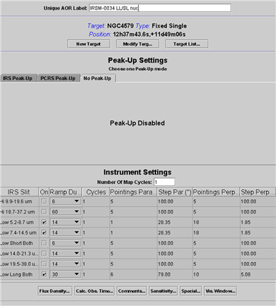
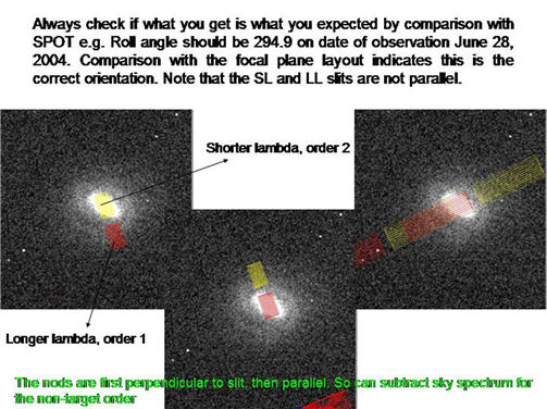
Before attempting any data reduction, visualize your AOR in Spot to understand the orientation of the observations and the sequence in which the files were generated. The AOR used and the visualization of these particular spectral mapping observations are shown below. As can be seen, the short wavelength modules each consist of 18 steps in the perpendicular direction while the LL1 module consists of 6 steps parallel to the slit and 10 steps perpendicular to the slit.
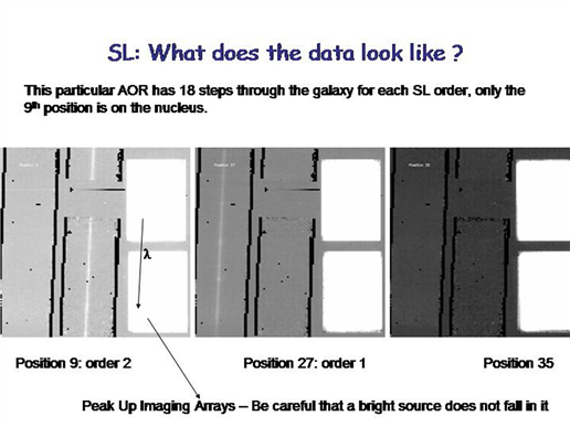
Now view your data in 2D format using your favorite fits file viewer such as DS9 or SAOIMAGE. The short-low data is shown on the left and the long-low data on the right for different positions in the spectral map. Note that in SL order 2, the nuclear source is in the slit in position 9. In SL order 1, the nuclear source is in the slit in position 27 for these observations.
14.4 Spectral extraction using SPICE
1. Launch SPICE. If SPICE is in your path, for example:
unix% spice &
2. Open a point source extraction flow in SPICE: File --> Open Spice Generic Template --> Point Source with Regular Extract.
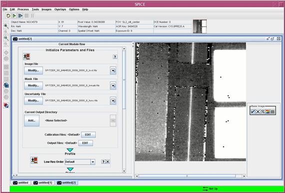
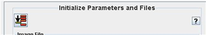
3. Load the BCD, uncertainty and mask files into SPICE. This is done by clicking on the "Modify" button for the "Image File" in the Initialize Parameters and Files module. If you are using archive file names, the corresponding mask and uncertainty files will be selected automatically. The BCD image will be displayed in the FITS window.
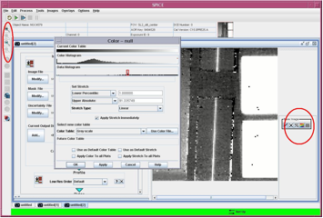
You can change the viewing parameters such as the stretch (using the controls on the right of the FITS window) or zoom of the display (controls on the left of the full SPICE window).
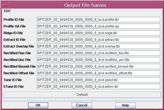
4. Check the name of the output files. Each time a module is run, the output files are overwritten, so you want to be careful in changing the output filename when you change the extraction parameters. First, select your output directory using the "Modify" button for "Current Output Directory". Next, you can review and modify the output file names using the "EDIT" button for "Output Files".
5. Run the Initialize Parameters and Files module. Click the "run" button in the upper left of the module.
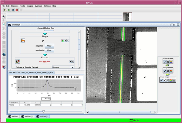
6. Run the Profile module. In this case, you do not need to change the Low Res Order of the profile. If there were an object in the non-target order (SL-1 in this case) you could change the order of the extraction. Again, run the module by clicking the "Run" button. The profile module collapses the spectrum in wavelength space for a particular slit order. This maximizes the S/N to help determine where the source is within the slit. When the module is run, the spatial profile will be displayed in the Plot window.
7. Run the Ridge module. If the "Percent Setting" is set to "Default" then the peak in the profile is automatically measured from the spatial profile by SPICE. This works well for bright, isolated, compact sources like the one in this example. Alternately, use the "Manual" option to enter a number as a percent of the slit width where the source should be extracted from. This is particularly useful when you want to extract the spectrum of the sky or the spectrum of a secondary source which is not the brightest source in the slit. The percentage appears as a dotted-blue line in the plot. Moving the line with the slider changes the percentage in the module, but moving the line by clicking on the plot does not. When you run the module, the trace and extraction width will be overlayed on the FITS image.
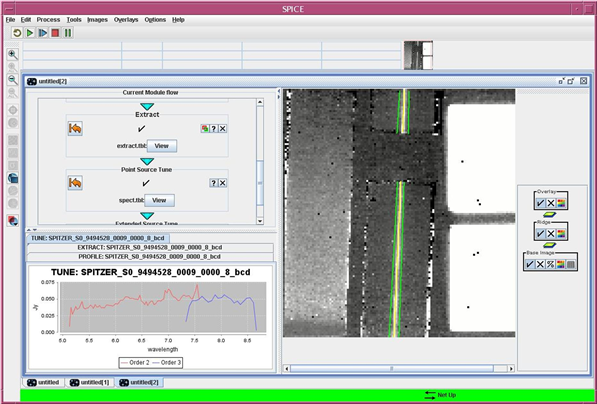
8. Specify the width over which the spectrum should be extracted. This can be re-defined in the next module, Extract. By default, an observation in SL-2 will be extracted as a point source with a narrow window which expands with wavelength. This default option is fine for the current example. Alternately, you can manually specify the width in pixels for a particular wavelength. The width of the extraction window increases with increasing wavelength to factor in the diffraction-limited point spread function. If you specify a width at 0 microns, then a constant width extraction window is used which is independent of wavelength. The overlay in the FITS window show which part of the slit is being extracted. In this module, there are also other options such as extended source extraction "ExtSrc", masking of specific bits and interpolation of NaNs which can help you improve the fidelity of your spectrum.
Run the module by clicking on the run button. The extracted spectrum will be displayed in the plot window in units of electrons per second.
9. Flux calibrate the extracted spectrum using Point Source Tune. Click the run button for this module (there are no parameters) to obtain a flux calibrated spectrum for a point source. If you use the default options in each step of the process, the output of tune should be exactly the same as that of the post-BCD files that you downloaded from the Spitzer archive. The output of the module is a file called *spect.tbl unless you have changed the output file name.
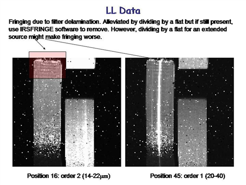
10. Remove fringes using IRSFRINGE. If you are working with LL data or high resolution data, it is likely that you will have residual fringes. This can be removed using the IDL procedure IRSFRINGE. Fire up IDL and at the IDL prompt:
IDL% irs=ipac2irs('spect.tbl')
IDL% irsd=irsfringe(irs,order=1)
IRSFRINGE has a number of different options which are discussed in the IRSFRINGE User’s Guide. These allow you to defringe only particular orders or a particular wavelength range or mask particular spectral features that might affect the defringing. Defringing is generally an empirical tool which should be used at the observer’s discretion since it is not always clear how many sine waves need to be fit to the data or what their relative frequencies are.
14.5 Miscellaneous Notes
SPICE will use calibration files which are consistent with the version of the pipeline that was used to process your data (see the CREATOR keyword in the header of your bcd.fits files). If they were processed with S11.0.2, SPICE will generate an error if you do not have the calibration files that correspond to S11.0.2.
SPICE has a batch mode which allows you to process large numbers of files in exactly the same way once you have identified the appropriate extraction parameters for your data. The usage is similar to the above example. Open the Batch flow using File --> Open Batch Spice Generic Template.
The default options for the steps outlined in this illustration i.e. profile, ridge, extract, tune and defringe will result in an output spectrum which is similar to the Spitzer IRS pipeline. You will want to improve the quality of your data before undertaking these steps by performing:
1.Sky subtraction: The pipeline post-BCD sky subtracted product is just one nod position from the other. You may want to create a supersky by taking a median of the BCD files from the off source position and subtract it from the on source data.
2. Creating bad/hot/rogue pixel masks: You may need to make new masks which are appropriate for your data by flagging bits in the bmask files.
3. Optimal Extraction: Improved S/N can be obtained for point sources using Optimal extract. This option runs a separate extraction module, which weights the extraction by the point source profile. Optimal extraction is documented in the SPICE GUI internal help pages. Open a separate optimal extraction flow from the file menu.
4. See the IRS Instrument Handbook which describes the steps you should undertake before publishing your IRS data.