Recipe 16. SPICE: Spectrum Extraction for Comet S-W 1
This demonstration uses SPICE to extract a spectrum from IRS data of the Comet Schwassmann-Wachmann 1. We describe the steps required to background-subtract your data and use the SPICE tool to perform a custom extraction of your target's spectrum. Background subtraction is particularly important for targets on a high background, such as that found in the ecliptic plane. Similarly for a moving target such as a comet, a custom extraction, rather than the standard pipeline product, may be important to separate the effects of nucleus and coma, and to otherwise correctly extract a slightly extended object, or one with an unusual morphology. This demonstration then, serves as a generic example for handling moving target data obtained with Spitzer IRS-Staring Mode. This specific example involves an extraction from the LL2 module, but it is generally applicable to all of the IRS modules.
2. Download the BCD and post-BCD data associated with the observation of Comet Schwassmann-Wachmann-1 in AOR 6068992. See Recipe 1 for instructions on how to download the data.
16.2 Step-by-Step Guide:
1. Perform the background subtraction. For IRS staring data in LL2, for point sources and slightly extended objects, this is simply done by subtracting the 2-D data from one nod position from the other. For most datasets, you may be able use the *bksub.fits spectra from the pbcd/ directory in your data extracted from the archive. These files are difference of the stacked (*coad2d.fits) products for each nod position). For the data in this moving target example, there are no *bksub.fits products so we will do the background subtraction by hand. This may be useful in other cases, if you have futher pre-processing you would like to explore.
;idl program to perform sky subtraction on IRS data
You can coadd the invidual DCE's yourself (taking care that you coadd only those exposures at a given slit nod position). There is no Spitzer-specific tool to do the sky subtraction, and we suggest you use your favorite data-reduction software to do this, ensuring that the sky-subtracted output is written out as a FITS image (and retains the FITS header corresponding to one of the DCEs at the proper nod position). For example, in IDL:
2. Launch the SPICE GUI. For example from the UNIX command-line:
unix% spice &
Within the SPICE GUI, open a point source extraction flow using File --> Open Spice Generic Template --> Point Source with Regular Extract.
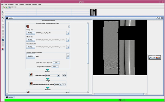
3. Load your data into SPICE by specifying the input data directories and names in the Initialize Parameters and Files module. Begin by clicking the "Modify" button for the "Image File". Provide the input background-subtracted 2-D spectral image (which you created in step 1), and the corresponding uncertainty image, and mask file. Normallly, the corresponding mask and uncertainty files will be automatically selected, but we have made our own image file, so we must enter them manually. If you used the *coa2d.fits files to create your sky-subtracted 2-D image, then use the c2unc.fits and c2mask.fits filed from the pbcd/ directory for the positive nod position, as your uncertainty and mask files for the sky subtracted data.
You can change the contrast ("stretch") of the 2-D image you are viewing using the color-grid button on the left of the FITS window, and using the display functions.
4. You can check the calibration files which SPICE will use with the "Calibration Files" button. Normally, you will allow SPICE to auto-select the pipeline version. Alternatively, as shown below, you can point SPICE to the custom calibration (CAL) files if you are an expert IRS user or if SPICE updates fall behind releases of new calibration by the SSC.
5. You can select the output directory and the names of the output files, using the corresonding "Modify" and "Edit" buttons in the input module. The output *.profile.tbl, *.ridge.tbl, *.extract.tbl, and *.spect.tbl files generated by the extraction will be written to the specified directory. The ultimate output table of interest is the *spect.tbl -- this is your extracted 1-D spectrum in (ascii) IPAC table format. These files will be overwritten if the flow is rerun, so you may wish to change the output file names if wish to have multiple versions in a common output directory.
When you have set all the input parameters, run the Initialize Parameters and Files module, using the run button in the upper left of the module window.
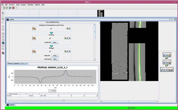
6. To begin the extraction, Run the Profile module, which calculates the wavelength-collapsed average profile in the spatial direction across the 2-D background-subtracted spectrum. (Although it is not appropriate in this example, the Profile module can be set to the non-target spectral order instead of using the default, which would then be the one extracted). Note that for the background-subtracted spectrum, a "positive" profile and a "negative" profile (from the other nod) relative to the zero level, are seen as the output. Next, establish the (peak) ridgeline of the spectrum in the dispersion direction along the 2-D spectrum by running the Ridge module. You can either allow SPICE to automatically derive the ridge peak or set the ridgeline peak manually by using the slider on the profile plot or typing into the box provided (clicking on the plot will move the dotted percentage line but not change the value in the box). When the module is run, the ridge line and the extraction window will be overlayed on the FITS image.
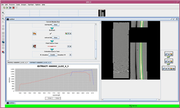
7. To extract the spectrum, run the Extract module. The extraction can be done with "Default" settings. For the low-resolution modules, the spectrum is extracted along the Ridge location, in accordance with the wavelength-dependent Point Spread Function (PSF) and the spectral trace (with "Auto" width). Alternately, the Extract function can employ a window with a different width ("Manual" width), but the width will still scale with wavelength, unless a full-slit extraction ("Full" width) is specified (using the ExtSrc option under ‘‘Width"). Note here that an ‘‘extended source" is expected to fill the entire slit. Although it is possible to manually set the extraction width (e.g. change it to 7 pixels at 14 microns) to pick up the comet’s coma, the default flux calibration in the subsequent step will not be accurate. Note that the output of the extraction is still in instrumental units, i.e., electrons/sec, and we perform the conversion to flux in the next step.
8. You still need to "tune" the extraction by applying the flux conversion from instrumental to absolute flux units. To do this, run the Point Source Tune module. Again, in this case the definition of an extended source is one that fills the entire slit so we use the Point Source function. The module corrects the slope and curvature of each order by applying the polynomial coefficients in the fluxcon.tbl calibration file. This correction is based on an order-by-order comparison of calibration data to standard star model spectra. The flux units are now in Janskys (Jy). Note that this conversion is only accurate for point sources and so will work for the comet nucleus, using the default ridge parameters. Currently, the tune calibration will not be accurate for extended targets that do not fill the slit, such as the nucleus + coma in this case. If you have MIPS or IRAC photometry of the same extended target you observed with IRS, it may also be possible to cross-calibrate the spectra using these imaging observations, as was done for the SW-1 observations (Stansberry et al., 2004, ApJS, 154, 463).
9. SPICE will output the profile, ridge and extract information, and the 1-D spectrum, as table files. This will go to the output directory you specified in step 5.
10. To quit SPICE, pull down the "File" menu and select "Exit."