Recipe 28. MOPEX/APEX: Point-Source Photometry at 70um
This recipe illustrates how to measure photometry for point sources from MIPS 70 micron images with uniform background. We show how to use APEX, a photometry package provided by the Spitzer Science Center. APEX is a part of a general package called MOPEX: MOsaicker and Point source EXtractor. We STRONGLY recommend that users check the intermediate outputs, either images or tables, generated by APEX. This allows you to decide if the APEX input parameters are appropriate for your specific data set.
It is important to note that this tutorial is specifically written for MIPS 70 micron data, which has unresolved point sources and uniform background. The recommendations from this recipe are applicable to data sets similar to those from the Spitzer COSMic Origins Survey (SCOSMOS). (http://irsa.ipac.caltech.edu/data/SPITZER/docs/spitzermission/observingprograms/legacy/) The SCOSMOS MIPS 70 micron data were taken in scan map mode with medium scan rate. The coverage per pixel is about 130-160. This type of 70 micron data were taken over a small area (0.25sq deg) in Spitzer Cycle 2, and were taken again over the full 2 sq. degrees in Spitzer Cycle 3. We use some of the Cycle-2 data for this recipe.
28.1 Requirements
You must have MOPEX (http://irsa.ipac.caltech.edu/data/SPITZER/docs/dataanalysistools/tools/mopex/) installed in order to follow along with this tutorial. MOPEX performs both image mosaicking and source photometry extraction. The source extraction part of MOPEX is called APEX. MOPEX/APEX can be used in either GUI mode or command line mode. For the first time users, we recommend the GUI version, which allows easy control and visualization of each processing step.
28.2 Download the example data
To follow the step-by-step instructions in this recipe, you will need to download the data set associated with Program 20070 (PI = D. Sanders). This program is Spitzer COSMOS (SCOSMOS) Legacy survey approved in Cycle 2. The MIPS 70 micron data were taken in scan mode. The final mosaic image was made by D. Frayer, a member of the SCOSMOS team, and a former member of the MIPS instrument support team. This recipe will use the data released by the SCOSMOS team via IPAC InfraRed Science Archive (IRSA). The data can be downloaded by going to http://irsa.ipac.caltech.edu/data/COSMOS/images/spitzer/mips/. From this link, you can download three images: mips_70_go2_cov_10.fits (coverage map), mips_70_go2_sci_10.fits (science image) and mips_70_go2_unc_10.fits (uncertainty image).
28.3 Extract Point Source Photometry
The primary purpose of this recipe is to present guidelines on how to extract point source photometry from a 70 micron mosaic with fairly uniform background. To begin, we recommend that users read the extensive documents on APEX software at http://irsa.ipac.caltech.edu/data/SPITZER/docs/dataanalysistools/tools/mopex/. APEX can provide PSF-fitted photometry as well as aperture photometry (circular apertures). Because MIPS 70 micron data has a PSF of roughly 16 arcsec (FWHM), PSF fitting does a better job in separating blended sources, and also can handle noise more reliably for faint sources than using aperture photometry. For these reasons, we recommend obtaining PSF fitted photometry if your targeted science data are point sources with moderate to low signal-to-noise.
28.4 Introduction: several important issues
� Point source Response Function (PRF)
When you download MOPEX, the MIPS 70 microns Point source Response Function (PRF) is a part of the package. This FITS file, mips70_prf_mosaic_4.0_4x.fits, is usually in a sub-directory called cal/. As its name indicates, this PRF was made for mosaicked 70 microns images. This PRF was made from a mosaic with a pixel scale of 4 arcseconds, generated from the Extragalactic First Look Survey (xFLS). It has a resampling factor of 4. It works well for sources of low and moderate brightnesses (<200 mJy). In addition, this PRF was derived to be large enough to go beyond the first Airy ring and its background was tuned to the zero level. If you use APEX for photometry extraction, you need to be sure that your 70 microns mosaic has the same pixel scale (4 arcsecond) as the PRF provided by APEX.
� Background
The second important issue to understand before running APEX is the background level in your mosaic image. This point is briefly mentioned in the previous discussion of the PRF. The principle is that whatever PRF you use has to be consistent with the mosaic image on which source extraction will be carried out. In addition to matching pixel scales as mentioned above, the background in the PRF image must match that in the mosaic image. The delivered 70 microns PRF image included in the APEX package was made to have a background level of zero. Therefore, users should ensure that within APEX the PRF fitting procedure is performed on an image which has a zero-background level. To achieve this goal, you can either directly input a background-subtracted image into APEX; or you can input a mosaic with non-zero background, then perform the background subtraction before measuring PRF-fitted photometry.
Here are the two ways to make background subtracted images from which PRF-fitted photometry can be measured:
1. Manually subtract the background before starting APEX : One can derive the background level by finding the median of the data distribution for source-free pixels within the mosaic. If one uses all pixels within a region, one can first apply multiple iterations of sigma rejection of outlier pixels before computing the median value. One can also fit a Gaussian to the central core of the data distribution after clipping off the wings.
2. Use the APEX module Extract MedFilter: It is possible to use this module to produce a reasonable background subtracted image for PRF fitted photometry. The trick is to make sure that the box size is big enough so that you are not including positive signals from sources, thus over-subtracting the background. With the SCOSMOS 70 microns data, we found that we can tune the APEX median filter parameters to produce acceptable background subtracted images. The specific values for the parameters in this module are discussed below.
For SCOSMOS data, we have tested both of these methods, and found very small differences. It is important to note that we run APEX Med Filter several times to identify the optimal parameters by comparing the results from both methods. For any other data, we strongly recommend users to examine the output from MedFilter , and make comparisons of results from two methods. It is important to be sure that the image used for the PRF-fitted photometry has zero background.
� Noise Map
In general, you will encounter three noise maps after you have used MOPEX to put together all individual exposures into a single mosaic.
The noise map with an extension of *_unc.fits is usually based on the SSC pipeline error propagation using individual bunc.fits images from the BCD products. The pipeline uncertainties were tuned to slightly under-estimate the true noise. This was tuned to be low to ensure that on-line pipeline processing can produce reasonable outlier rejection. We do not recommend to use this type of noise map for source detection and computing SNR.
The second noise image is measured by the standard deviation of the pixel stack at each sky position. This noise image is one of the outputs from the image mosaic tool MOPEX, and has an extension *std.fits. When your data set has good coverage, this type of noise map is usually much closer to the true sky noise level.
The third noise estimate is from APEX module GAUSSNOISE. This method involves measuring the pixel value distribution within a sliding box. In this method, the user can clip out a certain number of pixels whose data values deviate significantly from the median value. We will demonstrate the specific parameter settings in Section II. This noise image represents spatial pixel-to-pixel noise.
APEX uses noise images for two purposes: one is to determine the detection threshhold, another is to compute the signal-to-noise ratio for the PRF-fitted photometry. By default, APEX uses the noise estimated from the GAUSSNOISE module to determine sources above the specified detection threshold as well as for computing the SNR of the resulting photometry. The latest version of APEX also offers another option which allows users to choose a different noise image for SNR computation. This parameter is in the APEX single frame setting --- a switch allows one to use SIGMA_FILE to estimate SNR. This SIGMA_FILE can be defined by users to be any preferred noise map.
For the COSMOS data, we found that the noise image made by GAUSSNOISE is a little bit higher than mips_70_go2_unc_10.fits. In principle, if module GAUSSNOISE is properly tuned, its result should be close to the noise image measured from pixel stack (method 2 above). We recommend that users make comparisons among these noise images and make the appropriate selection for their own data. For the specific example here, we used the noise map estimated from GAUSSNOISE for detection and computing the SNR during the source fitting.
28.5 How to Run APEX
With the data set covering the full COSMOS area downloaded from IRSA, you can cut out the central region with deep data, and put a prefix 'sub' to all the file names. We run APEX with the following basic steps:
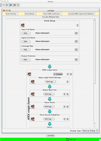
1. Start a new APEX single-frame pipeline. After starting up MOPEX, go to the main menu and select File-->New Apex Single-Frame Pipeline. In the window that pops up, select "APEX 1frame, MIPS 70 microns". The previously-empty MOPEX window will now be filled with a module flow consisting of "Initial Setup" and "APEX single frame". It will look like this:
2. Set parameters.
Only the parameters that require a change from the template default are listed below.
Initial Settings:
Input File Name mips70/sub_mips_70_go2_sci_10_0bck.fits
The background in this image has been manually subtracted and set to zero. See below for a detailed discussion.
Sigma File Name mips70/sub_mips_70_go2_unc_10.fits
Coverage Map mips70/sub_mips_70_go2_cov_10.fits
Output Directory mips70/apex_output/
Although we specify sub_mips_70_go2_unc_10.fits as the input noise map, during the extraction and SNR calculation, we recomputed noise within APEX using GAUSSNOISE module. For details, see below.
For our specific data set, we choose option (1), which allows the Detect module to directly run detection on it. With this option, you can directly fit the PRF to the image to obtain point source photometry. If you choose option (4), then APEX will need to subtract the background image. We have tested both options, and found that our manually background subtracted image produces slightly better (<2%) fluxes for bright sources than option (4), which uses Detect Medfilter to subtract the background.
For the shallow xFLS data, option (3), the filtered image, gives good results in detection, particularly for not producing false detections near bright sources. Option (4), PSP image, smooths data too much. A detailed discussion of the shallow data can also been found for the publicly released 70 micron image and catalogs for the xFLS data. Please refer to Frayer, D. et al. 2005, AJ, 131, 249. For the COSMOS data, where source blending is an issue, we use the input image without background subtraction since the filtered image can smooth out faint sources near a bright source. The down-side of this choice is that some false detections near most bright sources can not be avoided. These false detections can be cleaned up manually.
use background subtracted image for fitting = no
use data unc for fitted SNR = no
This option is set to no by default when you use GAUSSNOISE to estimate a better noise map for fitted SNR calculation. However, if you have a better noise map defined by SIGMA_FILE, you can set this option to yes for calculting SNR in the PRF fitting procedure.
Detect Med Filter Settings:
Window X (Y)
100 (100)
Outliers/Window
500
If the input image to the DETECT module is option (4), background subtracted image, then you need to run module Detect MedFilter to set the background level to zero before passing it to DETECT. Here is the explanation on how to set the parameters, and what we have tested for the SCOSMOS data set. This module produces a reasonable background subtracted image if the box size is set correctly. For MIPS 70 micron mosaic images featuring a pixel size of 4 arcsecond per pixel, one should use a box of 100 pixel by 100 pixel with the number of outliers set to 500. This rejects about 5% of bright pixels. This parameter is tuned for the moderate to deep MIPS 70 microns images taken by the SCOSMOS survey. The total integration time is about 1500 seconds. Boxes smaller than this will produce a background image with bright patches in regions with clusters of sources. This causes over-subtraction of the background for bright sources. This will affect the flux densities of bright sources at a level of a few percent. Obviously for shallower data with a lower surface number density of sources, the median box size could be smaller than what was used for the COSMOS data. Users need to experiment with their data to find the right parameters.
GAUSS NOISE Settings:
Window X (Y)
100 (100)
Outliers/Window
500
This module estimates the noise from a distribution of pixel values measured from a sliding box with a user-defined number of outliers. This noise image represents spatial pixel-to-pixel noise. By default, APEX uses the noise estimated from the GAUSSNOISE module to determine sources above the specified detection threshold as well as for computing the SNR of the resulting photometry.
DETECT
Detection_Max_Area
25
This is a number of pixels within the FWHM of the beam. Here we assume that the pixel size is 4 arcseconds. It is recommended that you set this value small to avoid breaking up individual sources.
Detection_Min_Area
6
We suggest that this parameter is not set to 1 to avoid spurious single pixel sources.
Extended_Object_Area
10000
You should set this parameter very large to avoid missing bright nearby sources by mistaking classifying the entire cluster region as an extended object.
Detection_Threshold
2.5
This threshold depends on the input image type and use_psp parameter. For the filtered and PSP images, one needs a larger threshold parameter than used for the raw image to reach similar source SNRs. We do not recommend digging too deep with APEX; we recommend only going deep enough to reach the desired depth in source SNRs such that number of sources in the raw extraction table is about 1.5--2 times that in the selected extraction table. If you set the threshold too low (APEX will take a long time) and can assign real source flux to nearby spurious noise peaks. If you set the threshold too high, then you can be incomplete at your selected SNR cutoff (e.g., when the raw table has a similar number of sources as your selected table).
Input_Type
"image_input"
We use Threshold_Type = 'peak'. This requires a pixel to be larger than the 8 adjacent pixels before declaring a detection (for Peaks_Radius=1). For close blends, the peaks of the fainter source(s) in the blend(s) may not be found. Also, APEX factors in the coverage map in determining whether a pixel is a peak (in rare cases the peak image pixel is not identified due to local variation of coverage).
Minimum Coverage
4
EXTRACT MEDFILTER
The parameters in this module are set with the same values as in Detect Med Filter
SOURCESTIMATE
Fitting_area_x/y
5
The units are pixels. This is set to be similar to the FWHM, so that APEX performs the fitting over a significant fraction of the area around the peak. If this parameter is set too low, there will not be enough pixels and APEX may derive a position off the real peak.
Max_Number_PS
1
This is set to 1 so that APEX fits only one source to each peak.
APERTURE PHOTOMETRY:
Number of Apertures
3
Number of circular apertures to draw around each source, between 1 and 5.
Aperture Radius 1, 2, 3
8.0, 10, 12.0
Radius of aperture N in pixels.
Inner and Outer Radius
15, 30
28.6 APEX parameters for COSMOS Data
Here we provide the exact parameters that were used for the COSMOS MIPS 70 microns mosaicked image. This set of parameters has produced a reasonable photometry catalog.