Recipe 31. GeRT: Correct Mild Saturation in MIPS-70 data
This recipe describes how to use the GeRT to recover mildly saturated sources in your MIPS-70 data. MIPS BCDs are created from the raw data cubes by calculating the slopes of the data ramps for each pixel. For more information about this, see the MIPS Data Handbook and Gordon et al. 2005 (PASP, 117, 503). Normally the BCDs use at least 4 samples to calculate the slope of the ramp, but if the pixel in question saturates before the last of these 4 samples, the pixel is flagged and masked in the BCD frame. The GeRT can be adjusted to re-make the BCDs using fewer samples, so, for example, pixels that are saturated at 4 samples, but not at 3, are recovered. The GeRT can generate BCDs using as few as 2 samples.
WARNING: changing the number of samples used to calculate the slope of the data ramp will affect the calibration of the data. You must read the 70 micron calibration paper (Gordon et al. 2007, PASP, 119, 1019) if you intend to use the GeRT to recover saturated pixels in your scientific data.
Obviously there are limits to the correction - pixels that are saturated before the second sample in the data ramps cannot be recovered, and so the GeRT can only work in cases of mild saturation. Here we describe how to re-create the BCDs using only 2 data samples to calculate the slope of the data ramp, so recovering the flux information from pixels that are mildly saturated in the postBCD image.
31.2 Inspect the Post-BCD mosaic to check for saturation
Download the example data via the link above, move the tarball into a clean working directory and unpack it. This should create 2 subdirectories labelled pbcd/ and raw/ containing the post-BCD mosaics and associated raw files from the Spitzer archive. The raw files provided in the tarball are a subset of the entire mosaic (to cut down on required disk space), so the final mosaic you create with these data will be smaller than the mosaicked image in the pbcd directory.
unix% tar xvf mips70_saturated_corr.tar
Open the MOPEX GUI and open the post-BCD mosaic, called pbcd/SPITZER_M2_20484608_0000_2_E3045040_maic.fits to see the final archive product (go to Image > FITS File Image). You can also do this in the image viewer of your choice (e.g. SAOImage DS9), but be aware that pixel NaN values (which show the position of the saturated data) show up as white in many viewers, rather than black (as in MOPEX) and so will not be immediately apparent.
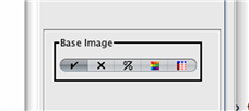
First we need to re-scale the image to see the saturated areas. Click on the little color palette in the "Base Image" control bar on the right hand side (4th button from left):
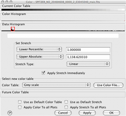
This will bring up a dialogue box. In the "Data Histogram" slider, drag the right-hand red bracket towards the left-hand side until you start to see the background detail appearing in the image.
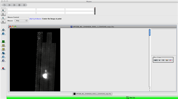
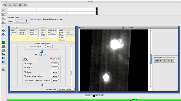
The MOPEX window should now look as follows:
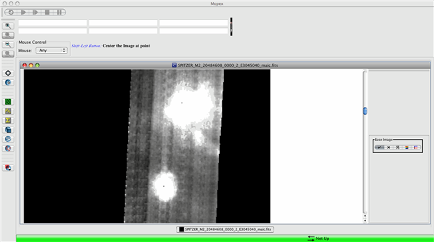
Now we need to find the saturated areas of the image. Scroll down the image to find the following two areas of extended emission. This image is zoomed in one level to show the saturated spots more clearly:
The small black spots in the areas of extended emission are areas of saturation. If you run your cursor over them, you will see that the flux value shown in the top left-hand corner of MOPEX disappears for those pixels (NaNs in the data). We will use the GeRT to re-make the BCDs to correct for these.
31.3 Setting up the GeRT input files
The GeRT needs two input files to recreate the BCDs from the raw data cubes. Firstly, we need to create a list of the raw data cubes to feed into the GeRT. Change into the raw/ directory and list all of the FITS files into an ASCII file:
unix% cd raw
unix% ls *raw.fits > rawlist.txt
Next we need to set up the GeRT to use only 2 data samples rather than the standard 4 to calculate the slopes of the data ramps. To do this we need to edit the file called MIPS70_SLOPE_0.nl found in the cdf/2/ directory of your GeRT installation:
unix% cd /your/GeRT/installation/directory/cdf/2/
unix% emacs MIPS70_SLOPE_0.nl
Scroll down the file until you find the parameter block starting with
&SLOPE
and change the following parameter from:
Min_Num_Samples = 4,
to
Min_Num_Samples = 2,
Important: your edits must include a space either side of the "=" sign, and must include the comma at the end of the line, else your changes will not be read.
In addition, we need to change the &CVTIN block to tell the GeRT to use all of the data, rather than rejecting the first frame in the data ramp:
&CVTIN
DataHi = 0,
DataLo = 0,
SatHi = 65500,
SatLo = 10,
StimHi = 4,
StimLo = 4,
&end
Once you have made these changes, save the file.
If this is the first time that you have used the GeRT, follow the setup instructions before going any further. The instructions can also be found in the GeRT installation directory (file called READme). Once the GeRT is set up, return to your working directory raw/.
unix% cd /where/you/unpacked_data/raw/
31.4 Running the GeRT
Once the input files are set up, you can run the GeRT to recreate the BCDs. From the directory containing the raw data, ensure that the GeRT is ready to run by sourcing the setup file, e.g.:
If you see any error messages then check the GeRT setup instructions to make sure that you have set the GeRT up correctly.
Run the GeRT to re-create the BCDs as follows:
unix% $WRAPDIR/gert.pl rawlist.txt ../OUTdir
where rawlist.txt is the list of raw files you created earlier, and ../OUTdir/ is the output directory. I chose to create the directory on the same level as the raw/ directory rather than as a subdirectory. This is not necessary, but comes in useful when trying to run MOPEX, as the file selection dialogue box in MOPEX takes a long time to show subdirectories if the directories contain a lot of files. The output from the GeRT should look something like this:
GeRT S14.0 v1.1 with 0 threads
0001 <* SPITZER_M2_20484608_0000_0033_2_raw.fits
0002 : SPITZER_M2_20484608_0000_0034_2_raw.fits
0003 : SPITZER_M2_20484608_0000_0035_2_raw.fits
0004 : SPITZER_M2_20484608_0000_0036_2_raw.fits
.......
.......
0291 : SPITZER_M2_20484608_0003_0222_2_raw.fits
0292 : SPITZER_M2_20484608_0003_0223_2_raw.fits
0293 : SPITZER_M2_20484608_0003_0224_2_raw.fits
SLOPER Processing done. 293 dce's in 273 seconds.
CALER Processing done, BCDs in ../OUTdir/bcd processed in 29 seconds.
Total processing of 293 dce's processed in 302 seconds
Check to see that the BCDs have been created in the output directory:
unix% cd ../OUTdir
unix% ls
The directory listing should show a subdirectory for each processed BCD, alongside the final recreated BCD image files and associated filtered BCDs, masks and uncertainty files. e.g.:
unix% ls *.fits
OUTdir.0001.bcd.fits
OUTdir.0001.bmask.fits
OUTdir.0001.bunc.fits
OUTdir.0001.fbcd.fits
OUTdir.0002.bcd.fits
OUTdir.0002.bmask.fits
OUTdir.0002.bunc.fits
OUTdir.0002.fbcd.fits
OUTdir.0003.bcd.fits
OUTdir.0003.bmask.fits
OUTdir.0003.bunc.fits
OUTdir.0003.fbcd.fits
.....
31.5 Re-Mosaicking the new BCDs
The final step is to use MOPEX to re-mosaic the new BCDs to check the results of the saturation correction. First we must create the input lists of images, associated masks and associated uncertainty files. List all of the *bcd.fits, *bunc.fits and *bmask.fits frames for input as follows:
unix% ls *.bcd.fits > imagelist.txt
unix% ls *.bunc.fits > sigmalist.txt
unix% ls *.bmask.fits > masklist.txt
Now remove all of the stim flash frames (all frames with header keyword STMFL70 = 1 are stim flash frames and should be rejected), and check that all of the data frames were taken with the 70 micron array as the prime array (PRIMEARR = 1; reject any frames with PRIMEARR = 2 or PRIMEARR = 3).
Once you have created the input lists, start the MOPEX GUI and load the Mosaic template for MIPS-70 data (go to File > New Mosaic Pipeline > Mosaic, 70 microns and hit "ok"). Set up the flow by setting the Image Stack File to point to the new list of BCDs, imagelist.txt, and choosing an Output Directory. Be patient when trying to load the Image Stack File - the directory contains a lot of images, and it can take a while for MOPEX to load the directory contents into the file selection window. Next you need to click on "Optional Input and Mask Files" and set the Sigma List File and the DCE Status Mask File to point to your sigmalist.txt and masklist.txt files, respectively. Again, be patient as it takes a while for MOPEX to display the directory contents. The Pmask FITS File should be set to the MIPS-70 PMask file found in the cal/ directory of your MOPEX installation (/your/mopex/directory/cal/mips70_pmask.fits) but the remaining input files can be left blank. Click "OK" and then start the flow running by clicking on the green "play" arrow in the top-left corner of the MOPEX window. Again, be patient when waiting for the flow to start.
Once the flow has finished, you should have a mosaic that looks like the one below, where you can see that the previously saturated areas of the extended emission regions now look good. REMEMBER - following this procedure will have affected the calibration of your data. Do not publish data processed in this way without first reading the MIPS-70 calibration paper (Gordon et al. 2007, PASP, 119, 1019).
Obviously, the background for this image is far from perfect, and additional processing will need to be done in order to correct for bad stim flash calibration and to refilter the BCDs to optimise them for photometry on extended objects. See the recipes ‘‘GeRT: Bad Stim Flash Correction in MIPS-70 data" and ‘‘GeRT: Filter Extended Sources in MIPS-70 data" for step-by-step instructions on how to do this. Refiltering the data to optimise for extended sources is only recommended if you are not interested in diffuse background emission such as the ISM.