|
IRS Features and Caveats
This page summarizes the most common features and artifacts see in IRS Peak-Up and spectroscopic data. We describe these features, show images with representative examples, and recommend methods for their removal from the data.
Contents
A. IRS Peak-Up Imaging
- Saturated Peak-Up Data
- Peak-Up Latents
- Rogue Pixels
B. All Spectral Modules
- Saturated Spectral Data
- Warm/Bad Pixels and NaNs in IRS Data
- Radhits on rogue pixels
- Severe Jailbars
- Latent Charge
C. Low-Resolution (SL and LL)
- Low-resolution non-repeatability
- Order Mismatches
- Curvature in SL1
- LL1 24 micron Deficit
- Incorrect Droop and Rowdroop corrections following peakup saturation
- Wiggles in Optimally Extracted SL spectra
- Residual Fringes in SL and LL
- SL14 micron Teardrop
D. High-Resolution (SH and LH)
- LH Tilts from Residual Dark
- LH Orders 1-3 Red Tilts
- High-res vs. Low-res spectral slope difference
- SH Spectral Ghosts
E. Solved Issues
- Bug in S18.7 High-resolution IRS Post-BCD products (solved in S18.18)
- Low-Res Nod 1 vs. Nod 2 Flux Offset (solved in S15)
- LL Nonlinearity Correction Too Large (solved in S14)
- Tilted SH and LH Flatfields (Solved in S14)
- Bumps in LH Near 20 Microns (Solved in S15)
- Mismatched LH Orders (Solved in S17)
- LL Salt and Pepper Rogues (Solved in S17)
A. IRS Peak-Up Imaging
1. Saturated Peak-Up Data
Saturated samples in the data can be identified in raw DCEs or in intermediate BCD products (lnz.fits or dmask.fits). The IRS uses a signed 16-bit A-to-D converter, resulting in a DN range for science observations of -32747 DN to 32767 DN. Therefore, in raw DCEs, saturated samples have values of 32767 DN. For data taken in DCS mode, like peak-up acquisition data, the range is 0 to 65535 DN.
Because the gain is 4.6 electrons/DN, saturated samples in lnz.fits have values typically above 298,000 electrons. This is slightly less than 4.6x216 because of dark current subtraction. Saturated samples have mask values in dmask.fits with bit #3 set. That is, the bit-by-bit logical "OR" operation of the sample mask value with the value 8 is non-zero.
The presence of saturated samples does not necessarily invalidate the data of the corresponding bcd.fits pixel because saturated samples in a ramp are excluded from slope calculations. Therefore, the reduction in the signal-to-noise ratio due to saturation depends on how many samples are saturated in the ramp. Bit #2 is set in bmask.fits for BCD pixels in which at least one sample of the ramp was saturated. Bit #13 is set if all samples of the ramp are saturated, and bit #12 is set if all but the first sample are saturated.
2. Peak-Up Latents
Bright objects falling on the IRS SL detector can result in persistent charge that appears as a latent image of the object in subsequent exposures. For exposures with (1-5)x104 electrons/pix in the last sample, 0.04 to 0.1% will remain behind as latent images in the subsequent exposure. These latents decay rather slowly, with an e-folding time of approximately 1100 seconds. For many successive exposures source flux can appear to increase by several percent. Given the parallel position of the peak-up fields-of-view to the SL slits, it is not uncommon for a bright object to fall on the peak-up arrays during science operations. Proper dithering strategies can mitigate the latent image problem, although with some loss of signal-to-noise on the affected pixels.
A second source of latent charge on the detector is simply the background. As a result, during very long Peak-Up Imaging AORs or those in very high background regions, the background level may be seen to rise slowly over time. This effect is stable and varies smoothly, so users may fit the (small) rise in the background and subtract it.
3. Rogue Pixels
A rogue pixel is a pixel with abnormally high dark current and/or photon responsivity (a "hot" pixel) that manifests as pattern noise in an IRS BCD image. The term "rogue" was used originally to distinguish pixels whose hotness was unpredictable, but now rogue pixel masks include those that are permanently as well as temporarily hot. At current bias levels there are very few rogue pixels in the peak-up windows. Proper dithering will mitigate the effect of rogue pixels, but they should be masked before mosaicking. See also Section B.2.
B. All Spectral Modules
1. Saturated Spectral Data
Please see "Saturated Peak-Up Data" above.
2. Rogue Pixels and NaNs in IRS Data
Rogue pixels are warm/unstable pixels. Early in the mission, all four IRS arrays were subjected to powerful solar proton events that deposited the equivalent dose of protons expected over 2.5 years in only two days. This damaged 1% of the SL and SH pixels, and 4% of the LL and LH pixels. See also Section A.3. The greatest science impact is to the LH module because the illuminated portion of the orders subtends only a few pixels in the spatial direction, making it more difficult to recover lost information by nodding the source along the slit. As the Spitzer cold mission progressed, the number of rogues and permanently damaged pixels increased. The bias for LH was lowered in IRS Campaign 25 in order to slow down the rate of rogue production at the expense of a decrease in sensitivity. Similarly, the bias and temperature were changed for LL in Campaign 45.
The damaged pixels are masked from data processing by assigning NaN status to them. This prevents numerical perations from being affected by their presence. Assigning any other real number would lead to improper processing of the surrounding signal information, such as during the extraction process. By default, the post-BCD EXTRACT module interpolates over the NaN pixels when adding flux within an aperture. The affected pixels are marked in the corresponding pmask and bmask.
Occasionally, it is possible for rogues pixels to propagate through the pipeline without being flagged as NaNs. In this case, these spurious pixel values will be extracted and appear as sharp spikes in the final spectrum. Such features should be readily recognizable as spectral features which are too sharp to be real. The IRSCLEAN_MASK package enables observers to visually inspect such pixels and interpolate over them. If there is any doubt about the reality of a given spectral feature seen in an extracted spectrum, we recommend that the observer always examine the 2D BCD images to confirm that the feature shows the expected spatial and spectral dispersion on the array.
3. Radhits on rogue pixels
Low and high resolution spectra may show a large spikes in places cosmic radiation hits (radhits) fall on highly-nonlinear (rogue) pixels. This effect is made more evident by the pipeline's (S15 and onward) rejection of samples following a radhit event. The early samples in nonlinear (rogue) pixels generally have steeper slope than the samples rejected after the radhit, increasing the flux after radhit rejection.
Rogue pixel data have incorrect values and should generally be filtered out before or during spectral extraction. Two methods can be used to remove the offending pixels:
1. Use SPICE to re-extract the spectra (using bcd.fits files as a starting point). Within SPICE you can use the Extract 'Mask' pulldown menu to mark bit 3. This will cause SPICE to ignore pixels with radhits. Then run Extract.
2. Use the IRSCLEAN routine to filter and replace the offending pixels.
4. Severe Jailbars
Very strong vertical stripes (jailbars) are seen in a single BCD image of an AOR. This may lead to very noisy or corrupted spectra.
A few rows of data in one plane of the corresponding cube will be seen to have anomalously high values (can be several tens of thousands of DN). These rows are not tagged as missing data, and in cubes of 4 samples, they are not recognized as outliers. Even before slope estimation, these rows affect the entire array because droop is impacted for all pixels of that plane, leading to severe jailbars.
The severe jailbars discussed here occur very infrequently (~1/700 DCEs). The root cause of the corrupted rows in the cube leading to severe jailbars is unknown. More mild jailbars may observed as a result of other causes.
There is no fix for this problem in the pipeline. It would have to be fixed at the raw datacube level. If multiple DCEs are available, throw out the offending DCE and recompute the spectrum.
5. Latent Charge
Despite the resetting of the detector after every integration, a small fraction of charge on the detector persists between frames. This latent charge is thought to be small, (~1-2% of the charge on the pixels) and decays slowly over time. It is removed by the annealing process which occurs every three to four days of an IRS campaign.
In the case of very faint sources, the source of latent charge is the zodiacal background. This charge can build up to significant levels over long integrations, sometimes as much as 30-50% of the true background in ~4 hour integrations. The slope of the latent build up is a function of wavelength and sky background but does not appear to be constant from AOR to AOR. The latent signal can be removed by fitting the slope of the background in each row (i.e. wavelength) as a function of frame number and subtracting that amount row-by-row from each frame. The slope can be fit by 1D or 2D polynomials and the fits should be visually checked to ensure that anomalous values for the sky have not been obtained. The figure below shows an example of the charge buildup in a long integration in a field with low (~18 MJy/sr) background as well as a 2D polynomial fit which was removed from each BCD at each wavelength. This effect should not be confused with the build up of charge and stabilization of signal discussed in Grillmair et al. (2007, ApJ 658, L115), when observations of a bright source are undertaken.
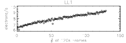
Latent charge buildup on the LL array during a long integration.
C. Low-Resolution (SL and LL)
1. Low-Resolution Non-repeatability
The one standard deviation repeatabilities of standard star flux measurements are: 4.6% for SL1, 2.2% for SL2, 3.1% for LL1, and 2.3% for LL2. These are for observations (AORs) that use high accuracy self-peakup. This is based on 129 observations of the standard star HD 173511 (see Figure below). Note that the distributions of flux values are non-Gaussian and that the SL1 distribution in particular has a tail of low flux values. The variations in measured flux are attributed to a combination of inaccuracies in telescope pointing (which can place the source away from the center of the slit) and flat field errors.
All spectrographs are susceptible to pointing errors. Flux calibrations are based on the median of all HR 7341 observations, so individual observations may give fluxes above or below the truth value.
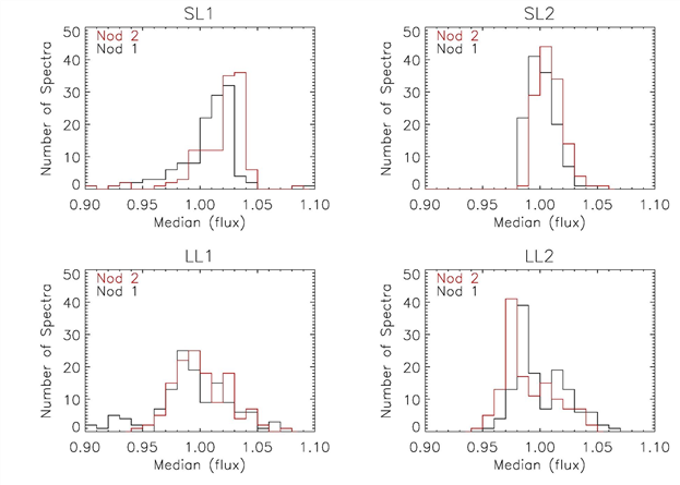
129 observations of the standard star HD 173511, processed using the S18.18 pipeline. The observations used high accuracy self peak-up. In each case the spectra have been normalized to the median of all fluxes at nod 1.
2. Order Mismatches
Depending on telescope pointing accuracy (see Caveat on Low-resolution Nonrepeatability), there can be mismatch between SL2/SL1, SL1/LL2, or LL2/LL1. See the figure below for an example of an SL1/LL2 mismatch. Such a mismatch could be mistaken as a broad spectral feature.
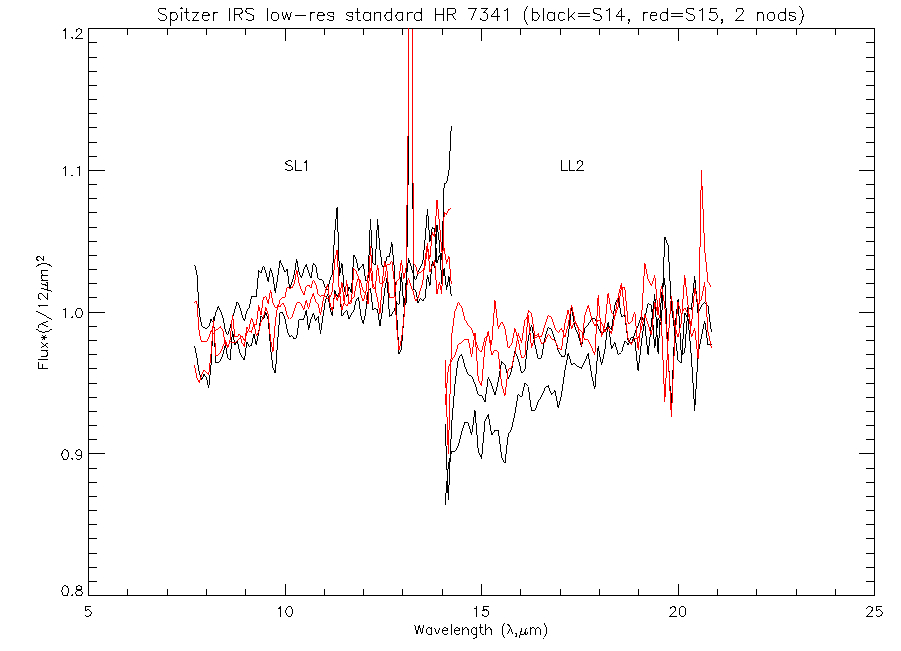
Order mismatch between SL1 and LL2, which might be mistaken as a broad absorption feature. For each order the two nods are shown.
Mitigation: Critically inspect all order matching. Individual orders that are low may be scaled up to match. Imaging photometry from IRAC, MIPS24, and IRS Peak-Up may be used to derive more accurate order matching corrections. However, see the caveat on SL1 curvature induced by wavelength-dependent slitloss.
3. Curvature in SL1
Spectral curvature (concave) may be induced in SL1 when the source is not centered in the slit, due to chromatic PSF losses. The curvature increases with apparent flux deficit. See the figure below.
Observers should be very wary of broad spectral features at levels <5%, especially at the order boundaries. The effects of the spectral curvature and order mismatch may be mistaken as broad absorption features.
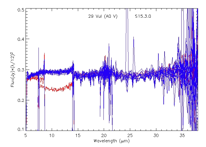
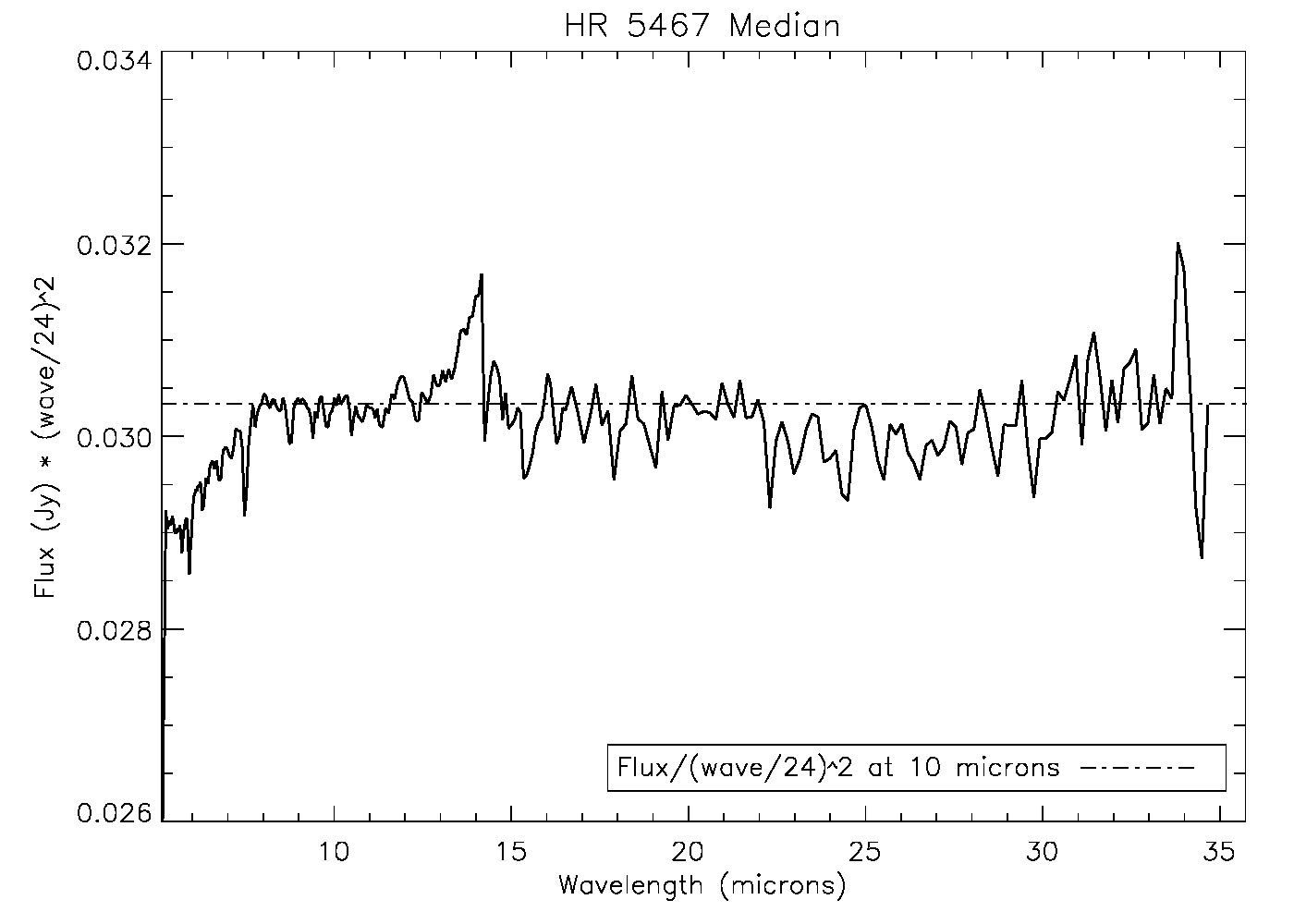
IRS Staring observations of 29 Vul, processed with S15 (bksub products). The red traces correspond to IRS observation campaign 7, while the blue correspond to five other campaigns.
4. LL1 24 micron Deficit
LL1 spectra of faint sources show a dip at 22-28 micron relative to standard models. (See the figures below for examples).The amplitude of the effect is 2-3% for faint (<80 mJy) sources. Some sources which show the deficit apparently have nonlinear ramps.
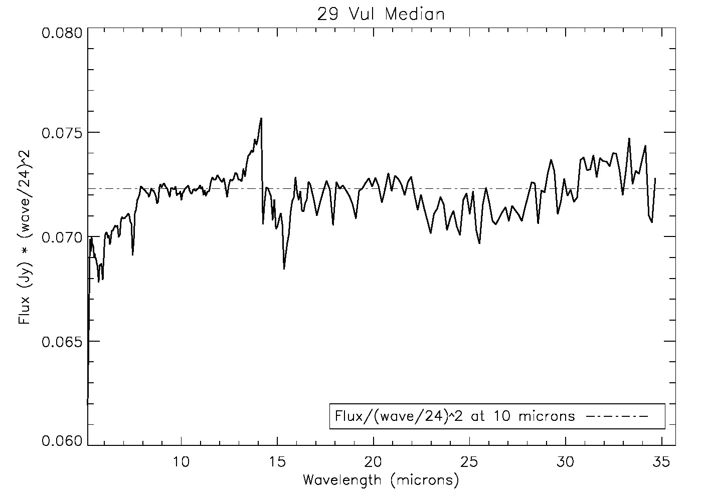
Illustration of the 24 micron deficit. The 14 micron teardrop is also visible.
Another illustration of the 24 micron deficit. The 14 micron teardrop is also visible.
5. Incorrect Droop and Rowdroop corrections following peak-up saturation
Spurious broad absorption or emission features or incorrect spectral slopes or curvature are seen in SL1 or SL2 spectra. This may be due to saturation of the peak-up arrays. SL exposures with long exposure times may saturate the peakup arrays. In cases of strong saturation, the droop and rowdroop corrections will be incorrect because the total charge on the chip (which determines the droop correction) and on each row (which determines the rowdroop correction) cannot be measured. The effect becomes worse as more pixels are saturated for a greater portion of the ramp. It may not be obvious from the image that the peak-up arrays are saturated.
6. Wiggles in Optimally Extracted SL spectra
Sinusoidal oscillations are seen in some high signal-to-noise SL spectra extracted using SPICE's 'Optimal' extraction option.
This effect is caused by a mismatch between the source and the standard star spatial profile (rectempl) file. The mismatch may be due to an incorrect 'Ridge' percentage or to undersampling of the PSF. The undersampling of the PSF in SL is evident in the BCD images as the source jumps from one column of pixels to the next, along the spectral trace. The locations of these jumps must match between source and template to get a clean optimal extraction. SL is the module most affected by undersampling.
To mitigate this effect,
- Use Regular extraction for high signal-to-noise data. Generally, if the S/N is high enough to see the wiggles there is little or no gain from using Optimal extraction.
- Compare Regular and Optimal SPICE extractions to verify the source of the wiggles.
- Manually change the percentage in 'Ridge' to minimize the wiggles. In general, automatic ridge finding is preferred for accurate ridge determination, however it is possible for the automatic procedure to miss the correct peak.
- Generate and use a standard star template (rectempl) that is a better match to the source. The template will match best if the position along the slit is the same (within 0.1 to 0.2 pixels) as the source position, modulo one pixel. For example, if the template is shifted by exactly one pixel, optimal extraction will work well, while if it is off by 0.5 pixel, the match will be poor.
- Try using the optimal extraction algorithm in SMART.
7. Residual Fringes in SL and LL
SL and LL spectra show residual (non-sinusoidal) wiggles after flat fielding, at the 1-2% level. The detector fringing pattern is sensitive to source location relative to the slit, which can be affected by pointing inaccuracies. In particular, the phase of the fringes changes with source distance from the slit center. The flat field has been constructed to accurately remove the fringes for the mean pointing at the standard nod positions. The residual fringes are non-sinusoidal, so IRSFRINGE does not do a good job at fitting and removing them. Users should critically assess the reality of spectral features at the 1-2% level.
8. SL 14 micron Teardrop
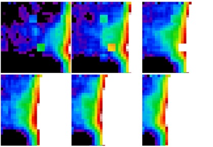
Excess emission is found in the spectral two-dimensional SL1 spectral images, to the left of the spectral trace, at 13.5-15 micron. We refer to this feature as the "14 micron teardrop", and it is illustrated in the figure below.
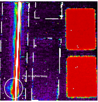
Example *bcd.fits image illustrating the 14 micron teardrop. The source was observed using SL1. The bright continuum can be seen running vertically down the image on the left. The white circle indicates the teardrop, which appears as a region of excess flux to the left of the continuum.
The following three spectra show what the teardrop looks like in the extracted spectra.
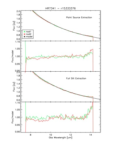
Illustration of 14 micron teardrop in the extracted spectra of HR 7341. The top two panels show the results for Regular Point Source extraction and the bottom two panels show the results for Full Width extraction. The teardrop is most clearly seen in panels 2 and 4, where it appears as an upturn kicking in at around 13.5 microns.
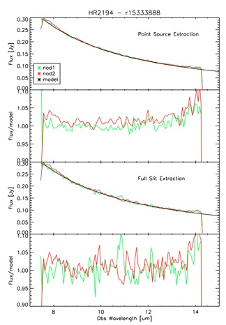
Same as figure above, but for HR 2194.
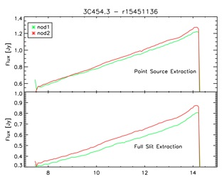
Similar to figure above, but for 3C 454.3, a red source. Comparisons to models have been omitted due to unavailability of models.
The teardrop is due to light leakage, optics, or detector response. It has not been introduced by pipeline processing. To illustrate this, the figures below show the various products from the pipeline for one observation of the standard star HR 7341. The teardrop is present in all of the pipeline products beginning as early as the Linearize cube.
LNZ Cube: Output of linearize � Frames 1-4.
After collapsing the cube above, the pipeline produces the following products:
Various pipeline products which all show the 14 micron teardrop: After the various droop corrections (top left); after stray light correction but before flat fielding (top right); after flat fielding (lower left); flat fielded but NOT stray light corrected (lower right).
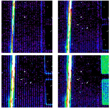
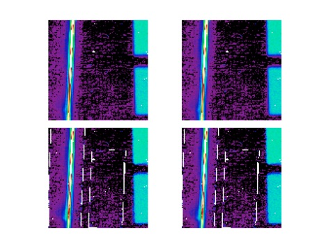
As illustrated the next three figure, the teardrop shape changes slightly with slit position, indicating that it is most likely correlated with the angle at which the light enters the slit, consistent with an internal reflection.
Nine mapping positions (2, 12, 22, 27, 32, 37, 42, 52, and 62) of the flat fielding data for eta1 Dor, zoomed in on the teardrop. The teardrop shape changes slightly with slit position, consistent with an internal reflection origin.
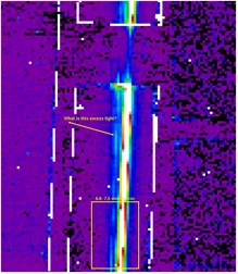
Two dimensional SL2 spectral image showing an observation of HR 7341. The wavelength region spanning 6.6-7.5 microns is highlighted with a box. We do not see any excess emission similar to the teardrop between 6.6 and 7.5 microns in SL2. This suggests the feature in SL2 at 6.5-7.6 microns is different in nature from the SL1 teardrop, and likely does not depend on extraction aperture.
In the figure below, we examine the strength of the teardrop versus the source flux density. We find that 1) the strength of the teardrop does not correlate with source flux density; and 2) for point-source extractions, the teardrop tends to be stronger for nod 2 compared to nod 1.
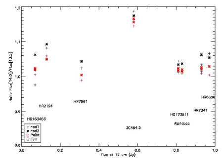
The strength of the teardop (quantified as the ratio of flux densities at 14.0 and 13.5 microns) versus the source flux density (measured at 12 microns) for 8 sources. For each source, black symbols represent full-slit extractions and red symbols represent point-source extractions. Plus signs represent nod 1 and asterisks represent nod 2. There is no correlation between the strength of the teardrop and the flux of the source. However, the teardrop is almost always stronger at nod 1 than nod 1 for point source extraction.
Mitigation: The behavior of the teardrop excess depends in a complicated way on source position in the slit and extraction aperture. There is no good way to correct for this feature. Users should use extreme caution before interpreting features between 13.2-15.0 microns.
D. High-Resolution (SH and LH)
1. LH Tilts from Residual Dark
During observations with the Long-High (LH) module, the dark current may have anomalously high values in the first 100-200 seconds of a series of exposures. Depending on the integration time and the number of cycles selected, data in the first exposure (or first nod position) may be affected. The "excess flux" is not evenly distributed over the LH array, being brightest on the blue end of each echelle order. The faint excess flux is seen as a bright band stretching across the bottom of the array, both on and between the orders, as illustrated in the figure below.
Illustration of excess LH dark current, which is distributed unevenly over the array with the brightest region towards the blue end (bottom) of the array.
This phenomenon manifests itself in extracted spectra of relatively faint sources as a "scalloping" or order tilting, wherein the slopes of affected orders are made bluer (flatter), inducing order-to-order discontinuities. The order-to-order discontinuities are typically 30-50 mJy. The magnitude of the effect does not seem to be related to source brightness. In the figure below, we show two extracted LH spectra of a faint point source. The top spectrum has the source at the nod 1 position, while the bottom spectrum has the source at the nod 2 position. A background sky spectrum has not been subtracted in either case, but the edges of the (color-coded) orders have been trimmed. The order mismatches are obvious in the nod 1 data, but vanish in the nod 2 data.
Nod 1 and nod 2 spectra. Notice the blue tilts in the nod 1 spectrum.
If you have observations of faint point sources with LH, and you are seeing these order tilts in your spectra, we recommend that you check your LH BCDs in the first nod position (or during the first few hundred seconds of a series of exposures), to see if this effect is more apparent. If order discontinuities such as described above are evident in the first few exposures or the first nod position, observers should consider not including these data during co-addition. If your LH data do not show this effect, you can include all the data in your final co-added spectrum.
Alternatively, users may wish to correct the effect using the DARK_SETTLE software. An example is given in the DARK_SETTLE recipe in the Spitzer Data Analysis Cookbook.
No similar effect has been conclusively identified in SL, LL, or SH modules. RED tilts of up to 10% have been seen in the longest wavelength LH orders 11 and 12, for bright red sources. This effect appears to be unrelated to dark current variations.
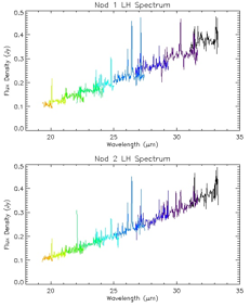
2. LH Orders 1-3 Red Tilts
LH orders 1-3 (at 29-37 micron) are sometimes mismatched and show red tilts with respect to shorter wavelength orders. The mismatch increases from 2% (order 3-4) to 10% (order 1-2). This effect appears to be most prominent for bright red sources (e.g., Mrk 231 in the figure below). It does not appear for bright blue stars, such as the primary LH calibration standard star ksiDra. The cause of these LH red tilts is unknown.
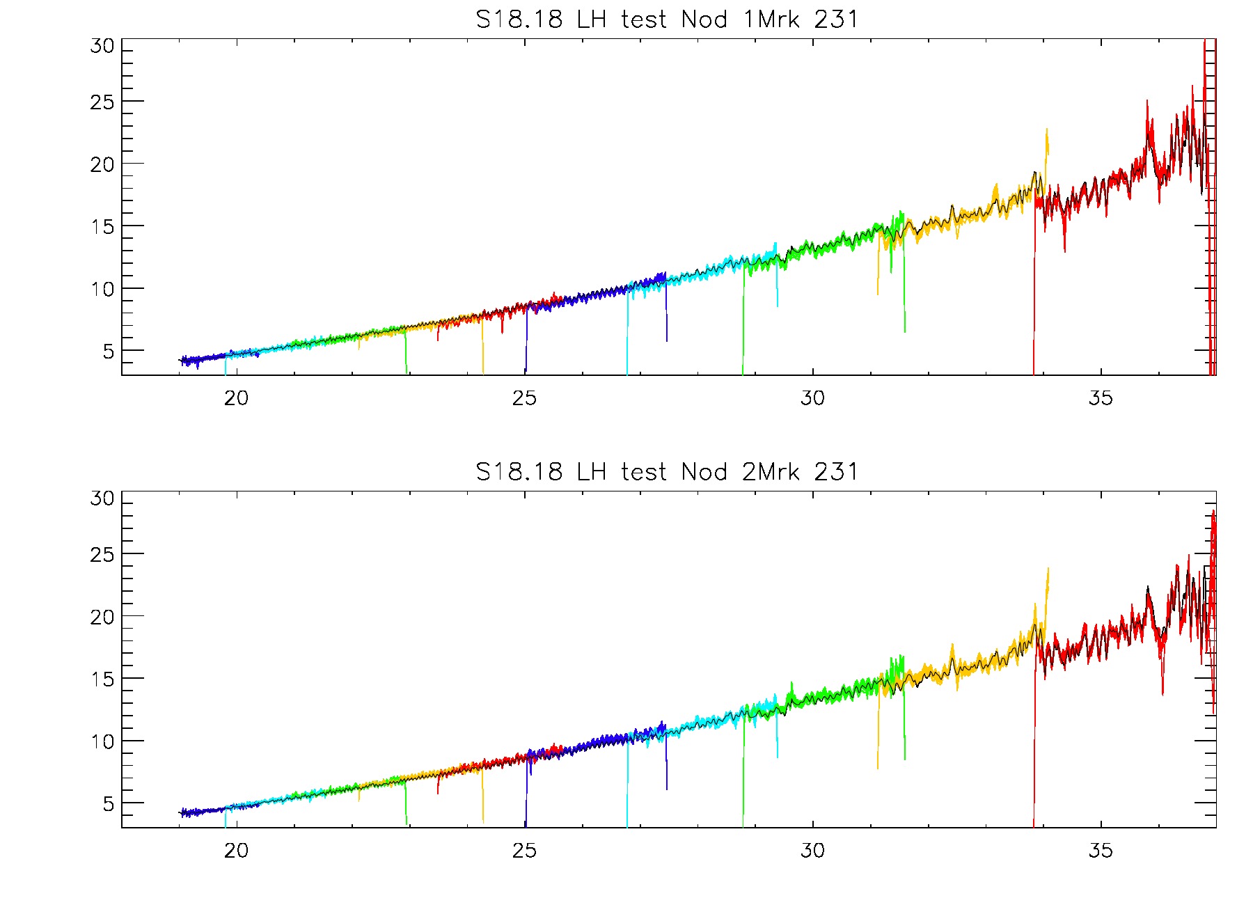
The LH spectrum of Mrk 231 shows red tilts in orders 1-3 (29-37 micron).
3. High-res vs. Low-res spectral slope difference
There is a small tilt of 2% over the 9-35 micron range of high-resolution spectra, relative to low-resolution spectra. Spectra match at 9 micron but LH is 2% higher at 35 micron than LL. Different standard stars and Decin models are used to calibrate LL and LH. HR 7341 (0.97 Jy at 12.0 micron) is used to calibrate LL. Ksi Dra (11.2 Jy at 12.0 micron) is used to calibrate LH. The 2% difference may be attributed to uncertainties in the fluxes of these two standard stars, which are of this order. Users may want to use broad band photometry to scale their spectra to the correct level.
4. SH Spectral Ghosts
"Ghosts" of extremely bright spectral lines can sometimes be seen in SH data, as illustrated in the figure below. These ghosts have an integrated flux of about 0.5% of the primary line in spectra extracted over the full slit. In the 2D spectra, the ghosts can have peak pixels that are about 1% of that seen in the primary feature. The ghost lines are off center to the left in the blue direction and to the right in the red direction, and partially overlap the slit edges. The separation of the ghosts from the line of origin increases with wavelength should not be mistaken for physical velocity structure in the target (the implied velocity if the ghosts were a physical structure ranges from 1800 km/s in order 20 to 2900 km/s in order 13 in the example shown in the figure). The ghosts are easiest to see in the 2D spectra, because they have a "tell-tale" spatial offset along the slit bracketing strong emission lines. Users who see very faint satellite lines around their emission features should inspect the sky-subtracted 2D spectra to determine if they are ghosts.
Ghost features are not seen in LH, and would be detectable if they had peak pixel values a few tenths of a percent of that in the primary feature.
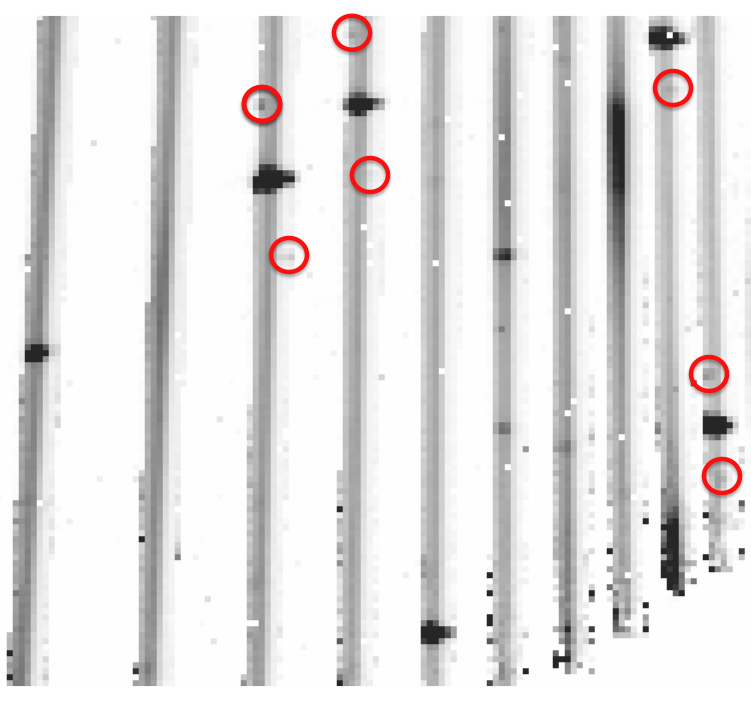
A bcd from AOR 16921344 of the planetary nebula J900. Red circles highlight the locations of the spectral ghost features.
Mitigation: Users concerned about removing these ghosts from their spectrum can easily do so by masking the pixels in the 2D image before extracting the spectrum.
E. Solved Issues
We include here issues that may be relevant for users that have data processed with older pipeline versions.
1. Bug in S18.7 High-resolution IRS Post-BCD products (Solved in S18.18)
As part of the standard IRS post-BCD data processing, all the BCDs associated with a given pointing are co-added. A bug in the pipeline sometimes causes incorrect weights to be used in the co-addition for S18.7 and earlier IRS high-resolution data. The problem occurs most frequently for SH data.
The affected files are all found in the "pbcd" directory of data sets downloaded from the Spitzer archive. Any of the co-added files ("coa2d.fits", "c2msk.fits", "c2unc.fits") may be incorrect. If a "coa2d.fits" file is found to be incorrect, any files generated from it will be also. The affected files have the following suffixes: "tune.fits", "tune.tbl". The BCDs are unaffected by this problem, so these files can be used to extract spectra and/or assemble spectral maps without cause for concern. To determine if your data are affected, please examine the "2dcoad.txt" files in the "pbcd" directory of your data set. The first column of this file contains the weights used in the co-addition. The weights should all be close to unity. If you see low and/or negative weights, then your co-added files may be corrupted.
The IRS team plans to reprocess all data in mid 2010, and this will rectify the problem. In the meantime, if desired, users can create their own "coa2d.fits" files by combining the appropriate "bcd.fits" files. The associated 1D spectra can then be extracted using SPICE. While it is possible to use a variety of software packages to create the co-added images, we are providing an IDL procedure for this purpose. This procedure, "coad.pro", can be found on the coad page Alternatively, users may co-add 1D spectra which have been extracted from the BCDs, which are unaffected by the bug.
2. Low-Res Nod 1 vs. Nod 2 Flux Offset (solved in S15)
SL Nod 2 fluxes are consistently 4% lower than Nod 1. This is the result of a spatial tilt in the flat field. LL2 Nod 1 fluxes are 4% lower than Nod 2 at 14-18 micron, decreasing to 1% at 21 micron. As a result, Nod 2 and Nod 1 are tilted relative to one another.
Users should average the nods to compute the source flux and determine the flux calibration. After S15, the flat field has been adjusted to remove the Nod1-Nod2 difference.
3. LL Nonlinearity Correction Too Large (solved in S14)
Slopes are overestimated at high count levels in LL. The effect is >5% for a 1 Jy source, and >20% for 2 Jy. The effect is worst for long exposure-times. SL nonlinearity correction appears to be OK.
Red sources appear redder and blue sources appear bluer due to this effect. However, curvature and other high order effects can also appear, reflecting the detector response. For example, fringes in the flat-field may be amplified, leading to extra 'noise' in LL spectra. The primary LL calibration source, HR 7341 (0.97 Jy at 12 micron) is affected by this problem at a low level. Reducing the nonlinearity coefficient causes a 5% drop in flux at 14-17 microns (LL2). The effect is <2% at 17-21 microns (LL2) and <1% at 26-36 microns (LL1).
To mitigate this problem, the non-linearity coefficient was adjusted for S14, resulting in a 5% drop in flux at 17-21 microns (LL2). This last effect has been corrected by revised flux calibration in S15.
4. Tilted SH and LH Flatfields (Solved in S14)
Before applying the fluxcon, the SH and LH orders appear tilted to the red. This is due to a difference between the standard extraction, which forces the wavsamp rectangle height to 1.0 pixels, and the custom extraction used to make the flatfield, which uses a variable height rectangle as defined by the wavsamp.
Pre-S15, the tilts were removed by applying the fluxcon table. From S15 onward, the variable height rectangles defined via the wavsamp are used for all extractions. This has the added benefit of matching the instrumental resolution.
5. Bumps in LH Near 20 Microns (Solved in S15)
Bumps are seen in LH orders 19 and 20, at ~19, 20, and 21 microns. They are attributable to bright features at the order edges which were accentuated by the S13-S14 LH flatfield. Features were not present pre-S13, and are fixed in the S15 flatfield. The pipeline S13.2 reduction showed three new peaks around 20 microns that are spurious. The features showed in a full slit extraction but when the extraction aperture is shrunk to 2 pixels, the feature vanished in one nod position but remained in the other. It is because of pixels X=13, Y=12 to 22, which all look unusually bright in the 2D frame even when the source is off on the other side of the slit.
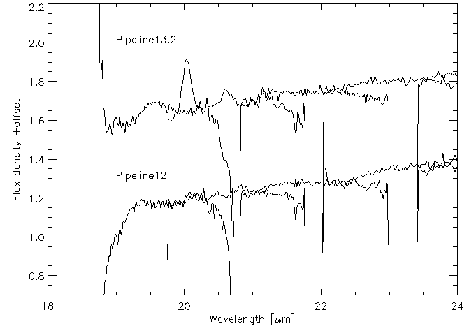
LH spectrum. Notice the peaks at 19, 20, and 21 microns in the S13.2 spectrum.
To mitigate this problem, a new LH flat field was created for S15, with bad regions suppressed. For S13, trimming the orders can remove the strongest of the three peaks but not its two weaker neighbors.
6. Mismatched LH Orders (Solved in S17)
For pipeline version S15.0, before flux calibration (in extract.tbl spectra), LH orders were mismatched and appeared tilted to the red. This was caused by the increasing wavsamp height with wavelength in each order to accomodate the spectrograph resolution. The effect was not apparent in the flux calibrated (spect.tbl) spectra, as it is corrected by the fluxcon polynomial.
For S17 onward, this effect is corrected at the spectral extraction stage. The flux in each wavelength bin is normalized to a wavsamp height of 1 pixel.
Note that this issue should not be confused with the LH blue tilts and red tilts discussed in D1, which still may be seen in some spectra.
7. LL Salt and Pepper Rogues (Solved in S17)
In S15, LL 'Super Darks' averaged over many campaigns were used to subtract off the instrumental bias signature. Due to the variable nature of rogue pixels, this introduced salt (new rogues not in the super dark), and pepper (rogues in the super dark, but not in the current campaign) into the data.
From S17 onward, campaign-dependent 'moving window darks' are used to better match the rogues in each campaign and to track the changing minimum zodiacal light level. The salt and pepper in S15 BCDs can be very effectively removed by subtracting an appropriate background observation.
|