III. 2MASS Details

3. Data Processing

b. Atlas Image Generation

The reduced R2-R1 frames for each 6°-long scan are spatially registered and combined into a series of 8.53´×17.07´ (512×1024 pixel, 1´´ per pixel) Atlas Images. The Atlas Images represent the coaddition of all six overlapping frames as described below. The images are centered on the cross-scan coverage, and adjacent images within a scan overlap in declination by 54´´. The J, H, and K_s band images are produced separately, but are registered onto a common astrometric grid to facilitate three-color investigations. Atlas Images are written in FITS format, and contain both the astrometric solution for the image in the J2000 coordinate system and the nightly calibrated photometric zeropoints within the FITS header (keyword "MAGZP"). Due to space limitations, the Atlas Images provided in the release data have been compressed using a lossy compression algorithm (hcompress).

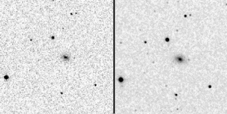
The Atlas Images are produced by first spatially registering the dark-subtracted, flattened, and sky-offset subtracted R2-R1 frames relative to each other, using the estimated positions of point sources in the frames (cf. IV.6). These frames are placed on the output Atlas Image coordinate grid one at a time, using a flux preserving interpolation kernel (see below). An example of a portion of a single frame along with the corresponding section of the combined Atlas Image is shown in Figure 1. Camera pixels which have poor responsivities, are excessively noisy, or are affected by transient effects, such as cosmic rays (as identified by unconfirmed single frame detections), are masked off during the interpolation procedure. Prior to adding the frame to the output image, the frame background is adjusted to match that of those frames already combined into the image, by removing the median of the differences at each point in the sky in the overlap region between the incoming frame and the previously-combined frames. This process produces seamless images, except in cases where the background levels vary rapidly with time due to clouds, atmospheric OH emission, or severe optical effects from extremely bright objects (such as beta Pegasi). The final output Atlas Image represents at each pixel the average of six such interpolated, background-adjusted frames. Because some pixels are masked, and there is some margin in the frame overlap, any one pixel in the Atlas Image may represent the average of anywhere from zero to seven frames. Output pixels consisting of zero or one frame are set to zero in the compressed Atlas Images.

Image Estimation Using Kernel Smoothing

The ideal image coaddition represents the best possible estimate of flux on the sky. Based on well-understood principles from density estimation {e.g., Density Estimation, B.W. Silverman 1986}, we smooth our square pixels to remove bias, but not so much that we introduce a large variance from the original images. The optimal smoothing balances these two sources of error.

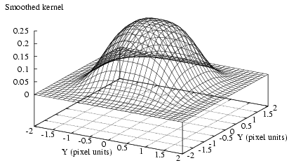
To derive a smoothing formula, we make the minimum knowledge assumption that a photon hits any point on the pixel with equal probability. We convolve our pixels with a Gaussian smoothing formula and adjust the smoothing length h to give optimal results.

Let be the smoothing kernel. This smoothing kernel is then integrated over the camera pixel to yield an estimate of the flux at points (x,y) for a particular pixel:

(Eq. III.3.b.1)

where (x_j,y_j) is the center of the j^th pixel with linear scale L=2´´. For convenience, we choose a Gaussian for the smoothing kernal K, which immediately yields:

(Eq. III.3.b.2)

The coadded flux estimate for n_pix pixels with value m is:

(Eq. III.3.b.3)

Given a coadd pixel of side length l and center at (x,y), the contribution from the frame pixel j follows by integrating Eq. III.3.b.2:

The mean integrated squared error,

(Eq. III.3.b.7)

where

is the estimate and f is the true flux density, is a standard measure for selecting the optimal smoothing length. Of course, we do not know the true f, but by taking the expectation of MISE, we can evaluate the first two terms from the data. Based on point sources, the optimal value for h=0.1. An empirical selection based on the pipeline performance on extended sources suggests h=0.35. Because the run of MISE for point sources slowly increases for values larger than the optimal, h=0.35 is still nearly optimal for point sources, and this value is adopted (see Figure 2).

Figure 1

Figure 2: Gaussian kernel with h=0.35 convolved over pixel with active linear size
L=1.0. The mesh diagram shows the contribution of the flux in the pixel centered
about the origin at arbitrary point (x,y).

[Last updated: 1999 May 4, by E. Kopan and M. Weinberg.]

Previous page. Next page.
Return to Explanatory Supplement TOC Page.