IV. 2MASS Data Processing

---

5. Extended Source Identification and Photometry

a. Introduction

The extended source sensitivity (10) is ~1 mag brighter than the point source limits, or 14.7 (2.1 mJy), 13.9 (3.0 mJy), and 13.1 (4.1 mJy) mag at J, H, K_s, respectively, with the precise threshold depending on the brightness profile of the extended source. Given the ~2´´ angular resolution of the image data and the detector sensitivity, 2MASS is well suited for detecting most types of galaxies to cz < 10,000 km/s and high luminosity giant galaxies beyond 30,000 km/s. In addition to galaxies, 2MASS will also identify compact and diffuse Galactic objects. The 2MASS catalogs are expected to detect over 100 million stars and greater than 1 million galaxies.

The scientific objectives of the extended-source portion of 2MASS include studies of large scale structure, utilization of the infrared Tully-Fisher relation, a complete survey of the local group of galaxies, and an unprecedented census of galaxies located behind the plane of the Milky Way, often referred to as the "Zone of Avoidance." As such, survey requirements were established in order to satisfactorily achieve these science goals. In addition to the sensitivity limits given above, the extended source Level 1 Specifications include >90% completeness and >98% reliability for most of the sky (free of stellar confusion). There are no set requirements for observations deep in the Galactic plane, but the survey maintains a high level of utility all the way down to |b| ~ 0° (Jarrett et al. 2000a, AJ, submitted). The Level 1 science requirements apply to the galaxy catalog derived from the 2MASS database.

The basic 2MASS data and pipeline reduction overview, including discussion of the point spread function - a basic component of star-galaxy separation - is given here. We also describe the key parametric measurements made on extended sources and the crucial operational step of background removal. In addition, we describe the algorithms developed to cleanly discriminate between point sources and extended sources. The catalog reliability criterion is, in particular, a difficult goal to achieve, necessitating implementation of algorithms specifically designed to perform star-galaxy separation with 2MASS imaging data. Finally, we give some examples of the wide array of extended sources that 2MASS detects. We will present more detailed scientific results from the 2MASS catalog, including galaxy colors, source counts, completeness and reliability, and clustering in a future paper, Jarrett et al. (2000b, in preparation).

b. Data and Basic Reductions

i. Image Data

The 2MASS survey strategy is to map the sky with overlapping strips, or tiles, each of approximately 6° in length and 8.5´ in width, using three (one for each band) 256 × 256 NICMOS (HgCdTe) arrays (2´´ pixels). The data are efficiently acquired with a freeze-frame scanning technique (detailed in Beichman et al. 1998, PASP, 110, 480), such that every piece of sky is observed a total of six times at 1.3 s of integration per sample. With careful sub-pixel dithering between samples, the deleterious effects of under-sampling are minimized. Frames are optimally combined to form "Atlas" images of size 512 × 1024 pixels with resampled 1´´ pixels; hence, 8.5´ × 17´ images. Each 6° scan is comprised of ~23 Atlas images. Atlas images have ~10% overlap, ~51´´, along the in-scan (declination) axis to minimize incompleteness of large galaxies. The Atlas image is the basic data product from which galaxies and extended sources are detected, characterized and extracted into the 2MASS database. In addition to the full Atlas images, small subsections of the Atlas images (referred to as "postage stamp" images) are extracted for each extended source (see below).

ii. Pipeline Reductions Overview

High level data reductions include linearity, dark frame subtraction and pixel-to-pixel gain correction (i.e., flat-field correction), which are formed in a non-standard fashion to accommodate the data set unique to the 2MASS survey (see the 2MAPPS Functional Design Document 1996; Beichman et al. 1998, PASP, 110, 480; Cutri 1997, in "The Impact of Large Scale Near-IR Sky Surveys"). Further pipeline reductions include frame-to-frame offset determinations, simple background subtraction, source detection, atmospheric "seeing" and point spread function (PSF) characterization, stellar photometry, band merging, artifact removal, accurate position reconstruction, and photometric calibration. The source detection step described below is vital to both point source processing and extended source processing. The extended source processing occurs at the end of the 2MASS data reduction pipeline. The main objective of the 2MASS extended source processor, referred to as GALWORKS, is to parameterize source detections and determine which sources are "extended" or resolved with respect to the PSF. Consequently, one of the many vital operations for successful star-galaxy discrimination is the accurate measurement of the PSF.

iii. Source Detection

The primary 2MASS source detection procedure is designed to locate both point sources (primarily stars) and extended sources (primarily galaxies). The detection thresholds are chosen to assure complete detection of galaxies brighter than the Level 1 specification, K_s ~ 13.5 and J ~ 15 mag, over a wide range in surface brightness. For fainter low surface brightness galaxies the completeness will steadily fall off with flux, hence a separate detection step is carried out to find these objects (see below).

The detection algorithm is closely modeled after the DAOPHOT FIND algorithm (Stetson 1990, PASP, 102, 932) which was devised to find stars over a wide range of stellar number density. Each Atlas image is convolved with a 4´´ FWHM Gaussian over a 13 pixel sub-array averaged to zero. The resulting zero-sum filtered image is set at a threshold of ~3 times the estimated noise level for the Atlas image, with detections corresponding to each central maximum within a threshold region. A rough position and flux is estimated from the corrected (convolved image) centroid. The detection list is then fed to a PSF characterization task (see below) and finally to a PSF profile-fitting photometry processor, where positions and integrated fluxes are refined. The detection thresholds (3) correspond to J~16 mag for point sources. For such faint sources, the implied extended source threshold is only ~0.5 mag brighter, producing a list of sources much fainter than the extended source requirements. Extended sources are ultimately identified from this inclusive detection source list.

iv. Data Anomalies and Artifacts

Data anomalies and image artifacts come in a variety of flavors, including those from the local environment (Observatory and atmosphere), space (meteor streaks, bright stars), from the equipment (array detectors and electronics, telescope tracking and focus), and from the software (algorithm and pipeline defects). Extended sources are vulnerable to most of these problems, but in particular those in which the image backgrounds are corrupted. For example, bright stars (K_s < 7 mag) induce several different image artifacts, including confusion halos, large-angular extent diffraction spikes, horizontal striping, persistence ghosting, reflection glinting, and large-scale background corruption for the brightest stars (K < 3 mag). Detection and removal of artifacts is a high priority in the reduction pipeline software and post-processing catalog generation. Still, it is not possible to eliminate all artifacts from the image and source products. Further discussion of data anomalies and artifacts is given below.

c. The Extended Source Processor

The last major subsystem to run in the 2MASS quasi-linear data reduction pipeline is the extended source processor, GALWORKS. The primary role of the processor is to characterize each detected source and decide which sources are "extended" or resolved with respect to the point spread function (PSF). Sources that are deemed "extended" are measured further and the information is output to a separate table. In addition to tabulated source information, a small "postage stamp" image is extracted for each extended source from the corresponding J, H and K_s Atlas images. The source lists and image data are stored in the 2MASS extended source database. The basic input/output flow is shown in Figure 1.

By the time GALWORKS is run in the 2MASS pipeline, point sources have been fully measured with refined positions and photometry, band-merged, coordinate positions calibrated, Atlas images constructed, and the time-dependent PSF characterized for every Atlas image. The high-level steps that encompass GALWORKS include: (1) bright star (and their associated features) removal, (2) large (>4´) cataloged-galaxy extraction and removal, (3) Atlas image background subtraction, (4) measurement of the stellar number density and confusion noise, (5) source parameterization and attribute measurements, including generation of PSF-tracking ridgelines, (6) star-galaxy discrimination, (7) refined photometric measurements, and finally (8) source and image extraction; see flow schematic in Figure 2. Additional post-pipeline processing are carried out to produce complete and reliable catalogs, which are released to the public.

Figure 1	Figure 2

2MASS is an all-sky project that will acquire something like ~40 Tb of data over the lifetime of the project. This places severe runtime restrictions on the pipeline reduction software; consequently, one important caveat is that most of the GALWORKS algorithms and flow structures were designed specifically to run and operate as fast and as efficient as possible, with some functionality omitted toward this end (e.g., orientation modeling). The background subtraction operation is a particularly crucial step since both star-galaxy discrimination and photometry rely upon accurate zeroing, smoothing and flattening of the image background. This operation is described in detail below. Steps 4-6 are designed to isolate "normal" galaxies and other relatively high central surface brightness extended sources.

The 2MASS extended source database contains several classes of "extended objects," including real galaxies, Galactic nebulae and pieces of large angular-size sources, Galactic H II regions, multiple stars (mostly double stars), artifacts (pieces of bright stars, meteor streaks, etc.) and faint (mostly point-like) sources with uncertain classifications. For extended sources, the ultimate goal of the 2MASS project is to produce a reliable catalog of real extended sources, predominantly galaxies. It is therefore necessary for additional "post-processing" steps to eliminate artifacts and confusing objects like double stars. We discuss here and here in detail how the star-galaxy separation process is performed. For the GALWORKS processor, the emphasis is placed primarily on completeness; that is, we want to comprehensively detect and identify extended sources (especially galaxies) brighter than the Level 1 specifications limits of K_s ~ 13.5, H ~14.3 and J ~15.0 mag. Later in the (non-GALWORKS) post-processing operations phase the galaxy completeness is relaxed (but still within the Level 1 requirements) in order to achieve the desired reliability in the galaxy catalog.

There are other kinds of extended sources that 2MASS is capable of detecting, including bright Galactic young stellar objects (H II regions, T-Tauri stars, etc.), faint nebulae and low surface-brightness (LSB) galaxies. These objects tend to be relatively rare and/or constrained to relatively small angular-sized fields toward the Galactic plane (e.g., molecular clouds) and as such there are no set requirements for their detection completeness or reliability. A separate catalog of bright extended stars and faint LSB galaxies will be released at a later date. A description of the algorithm to detect stars with associated extended emission and the algorithm to detect low central surface brightness galaxies are described below.

i. Atlas Image Background Removal

In the near-infrared, the background "sky" emission has structure at all size scales, primarily due to upper atmospheric aerosol and hydroxyl emission (the so-called "airglow" emission; see Ramsey et al 1992). The OH emission is the dominant component to the J (1.3 µm) and H-band (1.7 µm) backgrounds, while thermal continuum emission comprises the bulk of the K_s (2.2 µm) background. The J and H images tend to have more background "structure," and at times of severe airglow, the background can have high frequency features on scales of tens of arcseconds that can trigger false extended source detections. For extended sources, the primary objective of the 2MASS project is to find and characterize galaxies (and other extended objects) smaller than ~3´ in diameter. We therefore attempt to remove airglow features slightly larger than this limiting size scale to minimize random and systematic photometric error from non-zero background structure. This demands a more sophisticated fitting scheme then median filter or grid techniques allow (used, for example, in SExtractor, from Bertin & Arnouts 1996, A&AS, 117, 393). For the most part, the background variation in a given image (8.5´ × 17´) is smooth enough that it can be modeled with a polynomial. A third order polynomial turns out to be a good compromise between a simple planar fit and a series of spline waves. The fitting procedure is first preceded by an image "clean" operation. Stars and catalogued galaxies are masked from the image. Very bright stars (K < 6 mag) require more complicated masking, including removal of their bright internal reflection halo, diffraction spikes, horizontal streaks, filter glints and persistence ghosts.

The background removal process is applied separately to each J, H, and K_s Atlas image. Given the 2:1 image aspect ratio, the "cross-scan" (E-W) length, ~8.5´, represents the maximum area that can be modeled. Accordingly, a cubic polynomial, ax³ + bx² +cx + d, provides an effective model for smooth background variations larger than ~2´ to 3´. Along the 17´ "inscan" (N-S) direction we subdivide the array into three sections, consisting of lower and upper 512´´ blocks, and a central 512´´ block. The central block acts as the "glue" that smoothly joins the boundaries of the two lower/upper background solution sections. The final 512 × 1024 pixel composite solution is generated from a weighted average of each 512 × 512-block solution. The median value of the composite background solution for each band is extracted and tabulated in the 2MASS database (and catalog), identified as "<band>_sky", where <band> refers to either the J, H or K_s Atlas image. The median value of the background solution local to a particular extended source is called "<band>_back" in the database. The average "noise" in the background-subtracted (and star masked) Atlas image is derived from the average of the 16% and 84% histogram quartile values in the pixel value distribution. In this way the derived "noise" is analogous to a 1- RMS measurement. The pipeline extracted parameter identification is "<band>_bkgnd_sig_his", representing the "noise" of the background-removed Atlas image.

The decomposition schematic for background fitting procedure is illustrated in Figure 3. The 512 × 1024 Atlas image is represented by a thick-lined rectangle. The image is separated into three 512 × 512 pixel sections. The image sections are then smoothed with an 8 × 8 pixel median filter, to minimize contamination from faint stars and point-like objects that escaped the masking "clean" procedure (see above). Using a least-squares technique, a cubic polynomial is iteratively fit with 3 rejection to each smoothed line within a section. The line solutions are used as input to the next step, where we fit a cubic polynomial to each column in a section, thereby coupling the line and column background solutions. The three section solutions are then joined with a (1/r) taper. Here r refers to the relative radial ("in-scan") difference between any two given section solutions. So for example, combining the lower and central sections at some point, Y' (which ranges from 256 to 512 corresponding to the overlap region) gives the respective weights [1 / | 256-Y' |] and [1 / | 512 - Y' |], and for the central and upper sections the respective joining weights are [1 / | 512-Y' |] and [1 / | 768 - Y' |], where Y' ranges from 512 to 768. With this technique we are able to smoothly combine the three independent solutions per Atlas image. Note however, the boundary solutions for the upper and lower blocks are better constrained near the center of the image due to the weighted addition of the central block solution image. Conversely, the background solutions are not as well determined at the upper, >896 pixel row, and lower, <128 pixel row, "in-scan" image extremes.

Representative performance of the background removal operation is shown in Figure 4. The image data comes from a not-atypical "photometric" northern hemisphere night. Note the significant "airglow" emission during the period that this data was acquired (see H-band, middle panels). The figures show the "raw" Atlas Image, resultant background solution and residual (background subtracted) image. The gray-scale stretch ranges from -2 to 5 of the mean background level (where is the background "noise" derived from the background-removed Atlas image pixel histogram; see above). The J, H, and K_s raw images reveal fairly low level (smooth, but non-linear) background variations, while the corresponding residual images show very little (if any) background structure. However, airglow emission is much more prevalent in the H-band, with size scales smaller than ~1´-2´, as evident in the residual image. It is this residual structure in the background (with amplitude >10% of the mean background noise) that can induce systematics in the photometry, parameterization (e.g., azimuthal ellipse fitting), and reliability.

For the case in which the airglow frequency of variation is higher than can be adequately removed, the resultant photometry (particularly at H band) is severely compromised. These data are given a lower quality score and are scheduled for re-observation if time permits. Inevitably, there will remain cases in which residual airglow in the background-removed images significantly distorts the H-band photometry (and possibly at J-band as well) but otherwise goes unrecognized in the quality review process.

Figure 3	Figure 4

ii. Source Positions

In addition to the coordinate position based on the PSF-fit operation, two additional "extended source" positions are computed. The first is based upon the peak pixel from the J-band image, where 2MASS is most sensitive (except when dust extinction is appreciable). The precision of the peak-pixel coordinate is limited by the 2´´ resolution and convolution method used to construct/resample Atlas images from raw frames. Based on internal repeatability tests and external comparisons with astrometrically accurate galaxy catalogs (see Jarrett et al 2000b, in preparation), these coordinate positions possess a RMS uncertainty of ~0.5´´. They are identified in the 2MASS database as "ra" and "dec". The second is based upon the intensity-weighted centroid of the J+H+K_s "super" Atlas image. The "super" centroid coordinate position is usually more precise since it applies a 2-D centroid to higher SNR data, but it can be more influenced by unusual morphologies and extinction. Based on repeatability tests, the estimated uncertainty of the "super" centroid position is ~0.3´´ for normal surface brightness galaxies. The database names are "sup_ra" and "sup_dec".

iii. Ellipse Fitting and Object Orientation

The 2MASS undersampling and runtime constraints limit fitting an ellipse to a single surface brightness isophote in each band. To minimize the effect of PSF elongation and to best approximate the mean orientation of the galaxy being measured, the isophote to be fit corresponds to a surface brightness ~three times the background noise (3). The precise isophote value is derived from preset surface brightness values, one for each band, that are chosen to match (in a statistical sense) an equivalent surface brightness of ~3. These values are 20.09 mag/arcsec² at J, ~19.34 mag/arcsec² at H and ~18.55 mag/arcsec² at K_s, each corresponding to about ~3 for typical background levels encountered in 2MASS. The isophote center is anchored to the intensity peak-pixel of the source, where no attempt is made to iteratively adjust the isophote central position. The resultant elliptical parameters, axis ratio (b/a) and position angle (), are meant to represent the object orientation. It is this orientation that is used as a template for elliptical-isophotal and Kron photometry (described below) and for symmetry parameterization (also described below).

Using only one isophote to represent the shape of a galaxy is clearly an approximation since galaxies can change orientation with radius. But, in the near-infrared most galaxies appear to have somewhat more consistent orientations and axis ratios at different radii owing to the relatively smooth distribution of stars that dominate the 2µm light and the decreasing importance of extinction at these wavelengths. Moreover, most 2MASS galaxies are small in size (~15´´ in diameter), so for our ~2´´ angular resolution, multiple fits are not especially useful.

In addition to requiring that the ellipse-fitting method run fast, it also must be robust in the presence of confusion from nearby sources (i.e., stars) and correlated noise features that form "extended" limbs and other disconnected extended features. We do this by carefully masking neighboring sources when the stellar source density is high (see below), and removing linear 1-pixel wide "limbs" that extend outward from the primary 3 isophote (note: a real "limb" associated with the galaxy will generally be wider than 1 pixel). Moreover, since the desired ellipse model is symmetric across the major and minor axes, it tends to minimize the effects of asymmetric features (such as the presence of a nearby source). A "clean" isophote is critical for reliable convergence to the actual object orientation.

Once we have isolated the 3 isophote belonging to the objective galaxy, it is a straightforward procedure to fit an ellipse to the data. We assume that the center of the isophote corresponds to the peak in the light distribution (i.e., the peak pixel). The desired ellipse is then fully described by the axis ratio, position angle and K_s-band semi-major radius. The identifier names in the 2MASS database are "<band>_ba", "<band>_phi", and "r_3sig", respectively. We derive these values by minimizing the function

(Eq. IV.5.1)

which describes the elliptical radial distribution of the 3 isophote given some (b/a, ) solution. If r^ij_iso refers to the semi-major radius corresponding to 3 isophote (i, j) pixel located (x, y) from the central peak pixel position, then the mean radial distribution of 3 isophote pixels is and the population standard deviation is . If the ellipse (oriented by b/a and ) is perfectly matched to the isophote, then the mean variance in r_iso is identically zero, and represents the ellipse semi-major axis, r_semi. But if the match is poor, then the variance is large, while the population mean can be large or small, generally resulting in a large ² value. Therefore, by minimizing the ratio of the standard deviation to the mean radius in the distribution, we arrive at the best-fit ellipse solution. In this fashion, the elliptical parameters are derived for each band. Due to the resolution and sensitivity of the survey, there are practical limits to which we can measure the orientation and size of a galaxy: the minimum axis ratio is floored at 0.10 and the minimum semi-major axis radius is 5.0´´ (see below). We will refer to Eq. IV.5.1 as the "goodness of fit" or "chi-frac" metric; the J and K_s-band database names are "j_chi_ellf" and "k_chi_ellf", respectively. The goodness of fit metric can used to indicate problems with the fit (due to stellar contamination or noise in the case of faint sources) or real asymmetry in the object.

An additional fit is performed on the combined (J+H+K_s) "super" Atlas image. In general, the "super" Atlas image has a higher signal-to-noise ratio than the individual fits. Accordingly, the derived "super" Atlas image orientation serves as the "default" shape for cases in which the individual band flux is fainter than: ~14.4 mag at J, ~13.9 mag at H and ~13.5 mag at K_s, or when the S/N ratio of the galaxy is less than 5.0, based on the R=10´´ fixed circular aperture photometry. For the case in which the derived semi-major radius is less than 5´´ or greater than 70´´, the source is assumed to be round and the axis ratio parameter is set to unity. For the case in which the derived axial ratio is less than 0.10, the ellipse fit parameters are set to the corresponding fit from the "super" Atlas image. Finally, the "super" Atlas image values are also used when the individual band fit for one reason or another is not possible (e.g., when masked pixels are present within 1´´ of the peak pixel). The database names are "sup_ba", "sup_phi", "sup_r_3sig", and "sup_chi_ellf".

A final note regarding the ellipse fitting operation relates to nearby-neighbor masking. Bright disk galaxies (K_s < 12.5 mag) in which the inclination is large (>40°), are apt to be "split" into multiple point sources by the initial source detector (discussed above). Consequently, we do not perform any stellar masking or subtraction specific to the ellipse fitting step, except when the stellar number density is high, >2000 stars deg^-2 for K_s < 14 mag, in which case it is more favorable to mask out nearby stars given the high probability of contamination. This ellipse-fitting detail should not be confused with the general GALWORKS procedure of near-neighbor masking prior to photometry or radial-symmetry measurements.

iv. Photometry

Given the assorted shape, size and surface brightness that galaxies exhibit in the near-infrared, a corresponding diverse array of apertures is used to compute the integrated fluxes. Contamination from stars within or near the aperture boundary is minimized with pixel masking-but still remains significant when the confusion noise is high. Flux from masked pixels is "recovered" with isophotal substitution, where the mean value of the elliptical isophote (based on the elliptical shape parameters, b/a and ) replaces the given masked pixel that the isophote passes through. More detailed discussion of stellar contamination and rectification thereof in 2MASS galaxy photometry can be found in Jarrett et al. (1996, in The Impact of Large Scale Near-IR Sky Surveys, p. 213).

The simplest measures come from fixed circular apertures. Fluxes are reported for a set of fixed circular apertures at the following radii: 5, 7, 10, 15, 20, 25, 30, 40, 50, 60, and 70´´, centered on the J-band peak pixel. (Note: the large set of apertures was chosen so that the user could generate a curve of growth to estimate the total flux). We report both the integrated flux within the aperture (with fractional pixel boundaries) and the estimated uncertainty in the integrated flux. The magnitude uncertainty is based solely on the aperture size and the measured noise in the Atlas image, which includes both the read-noise component and background Poisson component, as well as the confusion noise component, which becomes significant when the stellar source density is high (see Appendix B). The uncertainty does not incorporate other errors due to source contamination, background gradients (e.g., airglow ridges with a higher spatial frequency than the background removal process can handle; see above), zero-point calibration error, and uncertainties in the adaptive apertures (e.g., isophotal photometry, see below). A more detailed discussion of the 2MASS galaxy photometry error tree can be found in Appendix A. Contamination, confusion and masking flags are also attached to each flux. In the 2MASS database the photometry names are, for example, "<band>_m_10", "<band>_msig_10", and "<band>_flg_10", for the 10´´ radius aperture photometry, uncertainty and confusion flag names, respectively.

For the great majority of faint galaxies in the 2MASS catalog, small fixed circular apertures give the best compromise between increasing noise, due to confusion and missing flux in the faint outer parts of galaxies. In particular, the circular 7´´ radius aperture appears to have the optimum match with the coupling between the 2MASS undersampling and PSF elongation, with the H and K_s background noise, and with the size of galaxies fainter than K_s~13 mag.

Adaptive aperture photometry includes isophotal and Kron metrics. The isophotal measurements are set at the 20 mag per arcsec² surface brightness isophote at K_s and the 21 mag per arcsec² at J, using both circular and elliptically shape-fit apertures (see previous subsection). Kron aperture photometry (Kron 1980, ApJS, 43, 305) employs a method in which the aperture is controlled/adapted to the first image moment radius. The Kron radius, which is frequently used in galaxy photometry as a "total" measure of the integrated flux (Koo 1986, ApJ, 311, 651; Bertin & Arnouts 1996, A&AS, 117, 393), turns out to roughly correspond to the 20 mag per arcsec² isophotal radius under typical observing conditions. The minimum radius is set at R=7´´, due to the rapidly increasing (PSF shape and background noise) uncertainty in the isophotal or Kron radial measurement for radii smaller than this limit.

For purposes of computing colors, two classes of adaptive photometry are carried out: individual and fiducial. "Individual" photometry refers to the use of adapted apertures derived per band, which is useful for single-band limited studies. The 2MASS database names (semi-major axis radius, integrated flux, uncertainty and confusion flag) for individual Kron photometry are "<band>_r_e", "<band>_m_e", "<band>_msig_e", and "<band>_flg_e", for elliptical apertures, and "<band>_r_c", "<band>_m_c", "<band>_msig_c", and "<band>_flg_c", for circular apertures. Database names for individual 20 mag per arcsec² isophotal photometry are "<band>_r_i20e", "<band>_m_i20e", "<band>_msig_i20e", and "<band>_flg_i20e", for elliptical apertures, and "<band>_r_i20c", "<band>_m_i20c", "<band>_msig_i20c", and "<band>_flg_i20c", for circular apertures. Individual 21 mag per arcsec² isophotal photometry names are "<band>_r_i21e", "<band>_m_i21e", "<band>_msig_i21e", and "<band>_flg_i21e", for elliptical apertures, and "<band>_r_i21c", "<band>_m_i21c", "<band>_msig_i21c", and "<band>_flg_i21c", for circular apertures.

The real power of 2MASS data is having simultaneous J-K_s, J-H and H-K_s colors. Colors require a consistent aperture size and shape for all three bands, based on either the J or K_s isophotes, respectively referred to as the "J fiducial" and "K fiducial" photometry. For the brighter galaxies in the catalog, K_s < 13 mag, the "K" fiducial isophotal elliptical aperture photometry appears to give the most precise measurement (based on repeatability tests), but errors in the ellipse fit to the 3 isophote (see previous subsection) result in an uncertainty that is difficult to evaluate (see Appendix A). The adaptive circular apertures reduce some of that uncertainty, but do increase the overall noise, due to additional sky noise within the non-optimized aperture-resulting in a less precise, but more robust measurement. 2MASS database names (semi-major axis radius, integrated flux, uncertainty and confusion flag, respectively) for fiducial Kron photometry are "r_fe", "<band>_m_fe", "<band>_msig_fe", and "<band>_flg_fe", for elliptical apertures, and "r_fc", "<band>_m_fc", "<band>_msig_fc", and "<band>_flg_fc", for circular apertures. Database names for fiducial 20 mag per arcsec² isophotal photometry are "r_k20fe", "<band>_m_k20fe", "<band>_msig_k20fe", and "<band>_flg_k20fe", for elliptical apertures, and "r_k20fc", "<band>_m_k20fc", "<band>_msig_k20fc", and "<band>_flg_k20fc", for circular apertures. J-band fiducial 21 mag per arcsec² isophotal photometry names are "r_j21fe", "<band>_m_j21fe", "<band>_msig_j21fe", and "<band>_flg_j21fe", for elliptical apertures, and "r_j21fc", "<band>_m_j21fc", "<band>_msig_j21fc", and "<band>_flg_j21fc", for circular apertures.

Additional flux measures include the central surface brightness (peak pixel flux) and the "core" surface brightness (average flux over a 5´´ radius). Database names are "<band>_peak" and "<band>_5surf", for the peak and core surface brightness respectively. Finally, a "system" measurement is carried out in which no stellar masking is performed, nor any masking of flux from neighboring galaxies. The "system" flux indicates the total flux in and about a galaxy, so it will include the total light in closely interacting systems. A set of contamination flags supplement the system measurements: one indicating stellar contamination and the other neighboring galaxy "contamination." Database names are "<band>_m_sys", "<band>_msig_sys" and "sys_flg", for the integrated flux, uncertainty and confusion flag, respectively.

The extrapolation mags represent the "total" flux of the object. The (circularly-shaped) radial surface brightness profile is first fit with a two-parameter exponential function, deriving the scale length and modifier , according to Eq. IV.5.2 (below). The profile extends down to the 20 mag arcsec^-2 isophote (per band). The inner 10´´ radius is excluded from the fit due to the proximal effects of the PSF (hence, f₀ is set to the isophotal value at 10´´ radius). The exponential is then extrapolated from the Kron radius (R<band>c, corresponding to 2.5 times the first moment radius), down to four times the Kron radius, with a maximum of 80´´ in radius.

RJext	J extrapolation radius
Jext	J mag from fit extrapolation
RHext	H extrapolation radius
Hext	H mag from fit extrapolation
RKsext	Ks extrapolation radius
Ksext	Ks mag from fit extrapolation

The utility of the extrapolation mags is limited to galaxies larger than 10´´, but smaller than 80´´. For this size range, the average mag offset between the circular isophotal mags (20 mag arcsec^-2) and the extrapolated mags is 0.33 ± 0.12 (band independent). In other words, the extrapolated mags recover 30% of the flux that is "lost" in the noise. One should cautiously keep in mind that the actual offset is morphology-dependent.

A cautionary note: like all isophotes used in 2MASS pipeline processing, the magnitudes of the isophotal contour for the isophotal magnitude are uncalibrated to 10%-20% and may be adjusted by ~0.1 to 0.2 mag in the later calibration processing step. Consequently, the isophote at which the 2-D elliptical parameters are derived can vary from (in background noise units) ~2.6 - 3.7, depending on the calibration correction.

v. Source Parameterization

Characterizing the Point Spread Function

The first step toward discerning extended sources, including galaxies and Galactic nebulae, from point sources (mostly stars) is to characterize the point spread function accurately. The distinctive shape of the 2MASS PSF derives from a combination of factors: the optics, large 2´´ pixels (frame images), dithering pattern of the six frame samples that comprise the Atlas image, location of the source within the unit cell of dither pattern, focus, sampling/convolution algorithm to generate the Atlas images, and atmospheric seeing. As such, the 2MASS PSF corresponding to frame-coadded images is not well fit with a simple Gaussian function. It can, however, be adequately characterized by a generalized exponential function (see below) out to a radius ~2×FWHM, that makes effective star-galaxy discrimination possible.

The 2MASS PSF typically varies on time scales of ~minutes due to: atmospheric "seeing" and thermally-driven variable telescope focus. The 2MASS telescopes are designed to be mostly free of afocal PSFs (under most conditions), but 2MASS images can be slightly out of focus during periods of rapid change in the air temperature - conditions that generally only occur during the hottest summer months. Out-of-focus images have the difficult property of possessing elongated PSFs. Fortunately, under most typical observing conditions for the survey, the PSFs are symmetric throughout the focal plane. That leaves the atmospheric seeing as the primary dynamic to the radial size of the PSF. Given the exposure times per sample (1.3 s) and the six-sample co-addition (with optimal dithering to produce round PSFs), seeing changes result in a mostly symmetric "puffing" in and out of the resultant Atlas image PSF (the seeing "speckle" pattern is negligible given the 1.3-s exposure time per frame and the co-addition smoothing). We can represent the image PSF with the generalized radially symmetric exponential of the form:

(Eq. IV.5.2)

where f₀ is the central surface brightness, r is the radius in arcsec, and and are free parameters. This versatile function (cf. Sersic 1968), not only describes the 2MASS PSF, but it is also used to characterize the radial profiles of galaxies, from disk-dominated spirals ( close to unity) to ellipsoidal galaxies ( ~ 4, de Vaucouleurs "law"). It has even been used to describe less-defined morphologies: Binggeli & Jerjen (1998, A&A, 333, 17) successfully modeled the surface brightness profiles of cD and dwarf spheroidal galaxies with this method.

The Radial "Shape" of Galaxies and Stars

Although the generalized surface brightness function (Eq. IV.5.2) can be used to derive meaningful fit parameters for galaxies brighter than K_s ~ 12 mag, for fainter galaxies the fit parameters are heavily influenced by the PSF and image noise. Furthermore, due to the relatively small areal region of the fit (Eq. IV.5.2) to the radial surface brightness, typically only ~8´´ in radius to minimize the effects of background noise, scale-length and modifier exhibit a high degree of correlation, and hence individual values of these parameters are not meaningful or physically connected to the source itself. Nevertheless, the fit parameters have still proved useful to distinguish extended sources from point sources. In particular, the quantity (×) robustly measures the average spatial extent of a source. Resolved galaxies tend to have larger values of both and than stars, so the multiplicative join of the exponential fitting parameters amplifies the difference between point sources and extended sources. The (×) quantity, referred to as the "radial shape" (or in short, "shape"), is the fundamental parameter for distinguishing between isolated stars and resolved objects (e.g., galaxies). Its variant cousins (described in the next subsection) provide further power for discriminating galaxies from more complex point sources, including double and triple stars.

The "shape" is also used as the atmospheric "seeing" metric for 2MASS point and extended source data. The generalized exponential function (Eq. IV.5.2) is applied to all sources, and a robust "shape" value is derived from an interval of time by careful analysis (see below). Here the "shape" is analogous to a FWHM measurement for the time-variable PSF. Our ability to track the seeing on short time scales depends on the density of stars. The more stars available to measure a statistically meaningful value of the "shape," the higher the frequency of seeing changes that can be tracked. A reasonable shape value can be derived from a minimum of about 10 stars. Consequently, for low stellar-density regions, like the north Galactic pole (~300 stars per deg² brighter than 14 mag at 2.2µm) the seeing is tracked on time scales of about 30 s; for high density regions (>10⁴ stars deg^-2) is tracked on time scales of a few seconds. Experience has shown that the seeing can indeed significantly change on times scales as fast as seconds of time (see below).

Stellar Ridgelines and Tracking the PSF

As is the case for all ground based observations, the PSF changes with time due to the changing thermal environment and dynamic atmospheric "seeing". The stellar "ridgeline" refers to the mean values of the PSF "shape" during an observation scan (6° in length and about 6 minutes of real time). The stellar ridgeline provide two important pieces of information crucial to both "seeing" tracking and star-galaxy separation: (1) time-dependent PSF, and (2) the uncertainty or spread in the stellar PSF distribution. The spread is a combination of an intrinsic component arising from the pixel undersampling in the original frames and dither pattern for co-addition, and an environmental component-the short time interval from which the main "shape" is computed is subject to small but variable seeing and focus changes.

The mean "shape" is determined from an ensemble of isolated stars spatially clustered along the in-scan direction (the arrow of time). The sample population must be free of extended sources (galaxies) and double stars to be a meaningful measure of the PSF. We employ an iterative selection method that is keyed by using an initial boot-strap from the lower quartile of the total population histogram. Since isolated stars will have an inherently smaller "shape" value than extended sources (or double stars), the lower quartile (25%) is populated nearly entirely by isolated stars and the upper quartile will be contaminated by resolved sources such as double stars and galaxies. Hence, the distribution's lower quartile serves as a good first guess to the actual mean shape value of isolated stars. Once the lower quartile is identified, we can iteratively search a restricted range in the histogram to arrive at a stable and robust estimation of the true mean shape value for isolated stars. The initial restricted range corresponds -3 to +2 of the lower quartile, where is the RMS scatter in the "shape" value. In the first iteration we use an a priori determination of . For each iteration thereafter, we set hard limits of ±2. The final "shape" value corresponds to the median (50% central quartile) of the restricted histogram sample, and the to the RMS scatter or standard deviation of the population. The 2MASS database names are "<band>_sh0" and "<band>_sig_sh0", respectively.

For the time-variable "seeing", we use the ridgeline to characterize the radial extent of the PSF. Two very different examples are illustrated in Figures 5 and 6. The plots show the median "shape" values (large filled circles) along the scan. Extracted sources (including stars and galaxies) are denoted with small points. The approximate (Gaussian derived) FWHM of the PSF are also shown to give some idea of the angular scale in arcseconds and the approximate relation between × "shape" and the more standard PSF FWHM. Note that these two measures are not uniquely related, but instead provide a more general relationship. In Figure 5 we show the resultant ridgeline for a scan passing through the Hercules cluster of galaxies. The stellar number density is not large (Galactic latitude of Hercules is about 30°), but there are still plenty of isolated stars easily separated from the cluster sources which are located above the mean "shape" ridge of stars. The seeing is fairly stable for each band all throughout the 6° scan spanning ~6 minutes of time. The same cannot be said for the second case, Figure 6, which demonstrates both poor seeing conditions and very rapid changes in the PSF. Fortunately, the stellar density is relatively high in this field, ~4000 stars per deg², and the rapid seeing diversions are, for the most part, sufficiently tracked. Scans for which the seeing is poorly tracked or the absolute value of the mean scan seeing is greater than 1.3´´ (~PSF FWHM > 4´´) are considered low quality data and are in most cases scheduled for re-observation.

Extended sources lie above the ridgeline defined by stars. We can reliably begin to separate stars from resolved sources at ~2 to 3 times the spread in the "shape" ridgeline. More generally, we can assess the "extendedness" of a source by how far it lies from the stellar ridgeline. The radial "shape" (×), or simply SH, of a source is compared to the stellar ridge value, SH₀ , and an N- "score" is computed as:

(Eq. IV.5.3)

where SH₀ (t´) and SH₀ (t´) denote the time variable ridgeline value and its associated uncertainty and SH(t), the source value, with time t´ as close to real t as possible. The PSF ridgeline value is stable over all flux levels, so only one value is needed per time interval. The 2MASS database name for the SH "score" parameter is "<band>_sc_sh".

The SH uncertainty includes both measurement error and the intrinsic PSF spread. However, since SNR > 10 stars are plentiful in most areas, the measurement error is minimal compared to the real spread in the PSF. The uncertainty represents the RMS in the SH distribution, but the distribution has triangular-shaped wings (i.e., the scatter in SH falls off linearly), due to the undersampling (in the original frames) and sub-pixel dither to optimally coadd the frames into Atlas Images. Consequently, stars will not have SH values above a threshold of ~2· SH₀, but galaxies and other relatively "extended" objects (e.g., double stars) will have scores >2. In the following subsections we will describe how we separate real extended sources (e.g., galaxies) from false extended sources (e.g., double stars) using several different flavors of stellar ridgelines.

Figure 5	Figure 6

vi. Star - Galaxy Discrimination

The ability to separate real extended sources (e.g., galaxies, nebulae, H II regions, etc.) from the vastly more numerous stars detected by 2MASS is what fundamentally limits the reliability of any extended source catalog. Single isolated point sources represent the purest and easiest construct from which extended sources must be distinguished. More complicated constructs include "double" stars and "triple+" stars, these are generic labels that include both physically-associated multiple systems and (more likely) chance superposition of stars on the sky. The permutations and combinations of multiple-star characteristics (radial separation, flux difference, color difference, etc.) make them a challenge to separate from real galaxies. The surface density of stars and galaxies is illustrated in Figure 7. Double stars are less than ~2% of the total stellar count at high Galactic latitudes, but begin to dominate the total numbers for |b| < 5°. Even at moderate stellar number density, double stars are comparable in number to galaxies for typical 2MASS flux levels.

There are many competing methods for separating stars from galaxies (or more generally, "classification"), from the simplest classification and regression tree methods (CART; e.g., linearly measuring one attribute vs. another), to ² automated induction (CHAID), to the more sophisticated Bayesian-based methods (e.g., FOCAS; see Valdes 1982, SPIE Proc. On Instrumentation in Astronomy IV, 331, 465), decision trees (e.g., Weir, Fayyad & Djorgovski, 1995, AJ, 109, 2401) and neural networks (e.g., Odewahn et al. 1992, AJ, 103, 318; Bertin & Arnouts 1996, A&AS, 117, 393). Each method was designed in response to increasingly more complicated data sets. For 2MASS, we were faced with undersampled near-infrared images subject to a variable PSF shape that called for a special adaptation of these procedures.

Early experimentation with existing algorithms (e.g., FOCAS) were unsatisfactory due primarily to the severely undersampled 2MASS PSF, which changes over time scales of minutes. A critical issue for GALWORKS is to accurately measure and track the time-varying PSF (see above) while applying some simple CART-like rules to cull out most of the multiple stars and artifacts that mimic real extended sources. The resultant extended source database is approximately 80% reliable for most of the sky. In a post-processing phase, further refinements, including more complicated attribute combinations and decisions trees (see below), are used to produce the extended source catalog at a reliability of greater than 98% for K_s < 13.5 mag. Later we describe and discuss some of the more critical parametric measurements and decision tree operations utilized to that end.

Figure 7

Basic Object Characteristics

The shape parameter is an effective star-galaxy discriminator: isolated stars and "resolved" sources (e.g. galaxies, double stars) are differentiated. In Figure 8 we display the J-band SH scores of three kinds of objects that 2MASS commonly encounters: stars, multiple stars (double stars and triple+ stars), and galaxies. Stars occupy a locus about zero SH score (as a result of defining the stellar ridgeline), while multiple stars lie well above the ridgeline along with galaxies and other "fuzzy" sources. The number of stars displayed has been reduced by a factor of 10 relative to the other plots in order to show the scatter in shape for the ridgeline vs. magnitude. The SH score is very effective at separating isolated stars from galaxies at flux levels as faint as J~15.4 mag.

Other GALWORKS-derived image parameters that are also effective at separating isolated stars from extended sources include the first and second intensity-weighted moments (2MASS database name are "<band>_sc_1mm" and "<band>_sc_2mm", respectively), ratio of the central surface brightness to the integrated brightness ("<band>_sc_mxdn"), and differential areal measures (e.g., isophotal area; "<band>_d_area"). Unfortunately, like the radial SH parameter, none of these diagnostics can discriminate galaxies from sky-projected clusters (i.e., double and triple+ stars) to the degree necessary to meet the Level 1 requirements. Double stars are particularly vexing due to their sheer numbers at |b| < 20° (Figure 7). Double stars (and triple stars near the Galactic plane) are clearly the primary contaminant of the galaxy database. More intricate attributes are needed to exploit the differences between groupings of point sources and genuinely extended sources.

Figure 8

Multiple Star - Galaxy Separation using Symmetry Metrics

In the near-infrared, the observed morphology for galaxies usually has smooth radial and azimuthal profiles. Spiral galaxies have much more even light distributions in the near-infrared than optical because the absorption is greatly reduced and the emission is dominated by older stellar populations, including low mass dwarfs and red giants, which are less concentrated in spiral arms. Features commonly seen at the radio and optical wavelengths, including H II regions, supernova remnants and dust lanes, are generally difficult to detect in the near-infrared except in the nearest galaxies; Figure 9 shows a few large angular scale galaxies located in the Virgo cluster. Only the relatively rare cases of galaxies subject to strong tidal or hydrodynamical interactions exhibit significant asymmetry in the near-infrared bands.

In contrast, multiple stars, and in particular double stars, are not radially symmetric about their "primary" peak-pixel center. Here the primary center of light of a multiple star corresponds to the brightest member in the group, or more specifically, the peak pixel associated with the brightest star, but can be in between for pairs of stars of equal brightness. We should point out an important feature of GALWORKS: it does not assume that a resolved object (i.e., two or more detections in close proximity) is a double or triple star, since real galaxies may be also be multiply-detected (in particular, bright edge-on galaxies may induce several detections along its disk). Hence, we do not make a distinction between double stars that are resolved or unresolved with respect to the PSF. Instead, we must apply other tests to decide whether an object is truly "extended" or not. Below we describe the methods that are utilized in the pipeline GALWORKS software.

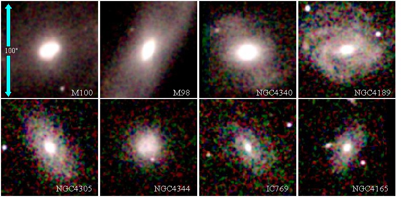
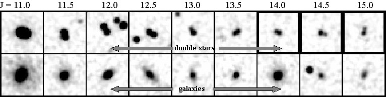
The near-infrared symmetry of galaxies can be exploited to differentiate between multiple stars that otherwise mimic extended sources. Figure 10 illustrates a variety of double stars seen in 2MASS images. For comparison, a set of galaxies of approximately the same integrated brightness as that of the double stars is also shown in the lower panels. Both sets of sources were classified using higher resolution (~1´´ PSF) optical imaging data and with the Digitized Sky Survey image data (see also below for a description of the "training sets"). Surface brightness profiles and colors distinguish true extended sources from point-like objects (in this case, double stars). For double stars, the fainter star ("secondary" component) breaks the symmetry about the primary. Hence, the signature of a double star is an asymmetric azimuthal profile.

Figure 9	Figure 10

So as not to enforce a strong bias against asymmetric or foreground-contaminated galaxies, the various "symmetry" parameters and metrics used to discriminate galaxies from stars (described below) are used judiciously in conjunction with non-biased parameters (e.g., SH). Here we employ two different strategies at forming symmetry parameters. The first is to exploit the measured 2-dimensional orientation of the source, and the second is to utilize the generalized PSF function (Eq. IV.5.2) under scenarios in which the degree of asymmetry in the object can be measured.

Once the general orientation of the galaxy is derived (see above), the "symmetry" of the object can be appraised. As discussed earlier, the radial and azimuthal symmetry of an object is a good indicator of its true nature. Double stars appear asymmetric across the minor axis-since the ellipse is centered on the primary component of the double star. This is also generally the case for triple stars, although there are maddening configurations of 3 stars in which the alignment is symmetric across both the minor and major axes.

One way to measure the "symmetry" of an object is to perform a bi-symmetric flux comparison between the two half-sides as defined by the minor axis (see above). Perfectly symmetric objects will have a flux ratio that is equal to unity. We may also cross-correlate the pixel-values in the two halves by simply rotating one side 180° with respect to the other and multiply the resultant pieces. The desired asymmetry "measure" is then the sum, normalized by the total integrated flux squared. To minimize the effects of noise and the shape of the PSF, very low SNR points (< 1.5) and the inner 3´´ core are avoided in this procedure. A more elegant variation on this method avoids the deleterious effects of low SNR points; namely, we perform the cross-correlation with a reduced ² function of the form,

(Eq. IV.5.4)

where p and p* are pixel values at points 180° apart, N is the number of points being compared, and is the pixel noise (but ignoring the noise contribution of photons from the source itself). This ² measure has the multiple advantage that it has a distribution that is well understood statistically with tabulated confidence ranges, there are no asymmetries in the distribution like those introduced in a ratio comparison, and it is insensitive to low SNR or data points near zero. The final symmetry measure comes from the object orientation "goodness of fit" parameter (Eq. IV.5.1). The 2MASS database names are "<band>_bisym_rat", "<band>_bisym_chi" and "<band>_chif_ellf", for the bi-symmetry flux ratio, cross-correlation and ellipse "goodness of fit" to the 3- isophote, respectively.

A different tactic is to "remove" the secondary and measure the resultant SH (Eq. IV.5.3) of the "deblended" primary. We are, of course, faced with the problem that the emission from both sources are entangled and the primary itself has changed both its radial (SH) width and its azimuthal (symmetry) shape. If the PSFs were exceptionally stable and well characterized as such, then in principle it would be possible to satisfactorily de-blend the multiple sources into their constituent parts. Since this condition is not always realized, and moreover the runtime for this kind of multiple PSF ² fitting is prohibitively long, we are left with less ideal methods.

The simplest approach is to remove the secondary using a median filter in annular shells about the primary: GALWORKS refers to the resultant measure as the "median shape" or MSH (in the database it is called "<band>_sc_msh"). A more satisfactory (if more complicated) approach is to mask the secondary and measure the residual emission from the primary, using a 45° wedge or pie-shaped mask that is rotated about the vertex anchored to the primary. The optimum configuration in which the secondary is effectively masked is found by rotating the wedge mask through all angles (Figure 11). The SH score is then computed for the remaining area (360° - 45°). If the secondary star is masked, then the resultant SH score will be minimized, ideally with a value corresponding to an isolated star. In practice the secondary can never be fully masked, and the peak pixel does not represent the true center of the primary since it is slightly shifted toward the secondary-thus resulting in a slightly inflated SH score relative to that of an isolated star. Nevertheless, the "wedge" shape score, or WSH (in the database it is called "<band>_sc_wsh"), is an effective discriminant. This is demonstrated in Figure 12, which is analogous to Figure 8; here we show the distribution of multiple stars and galaxies as measured in the WSH vs. magnitude plane.

The wedge shape score for double stars is considerably smaller than the corresponding SH score, having values typically less than 5 for J < 15 mag, while galaxies remain "extended" in this measure with scores >5 for J < 15 mag. Note however, triples+ stars are only occasionally identified as such by the WSH score since the additional two secondary components usually defeat the single rotating mask method. For triple stars, yet more severe "symmetry" constraints are required.

Triple stars are geometrically more difficult to characterize because of the number of possible combinations of integrated flux and primary-secondary separations. For most triple stars there is minimal contamination from the two secondary components along some radial direction from the primary. If we measure the radial SH of this vector and compare it to the corresponding ridgeline value, the resultant "score" should be close to that of an isolated star. Thus the basic method is to measure the SH along an azimuthally distributed set of vectors at angular separations of 5°. The vector corresponding to the "minimum" shape score (referred to as the R1 score; in the database it is called "<band>_sc_r1") is susceptible to background noise fluctuations since we are restricting the (, ) fitting operation to less than a dozen pixels. For galaxies, the R1 score tends to select against galaxies that are edge-on and thus have minimal (but still measurable) extended emission along the minor axis (i.e., the vector corresponding to the minimum radial SH score).

A more robust parameter, but slightly less effective at removing the influence of the secondary components, is to average the second and third lowest SH value vectors. This score is referred to as the R23 shape score (in the database it is called "<band>_sc_r23"). Here we are relying upon the fact that most triple star configurations (but not all by any means) will have more than one vector that is only minimally affected by the secondary components. Galaxies, meanwhile, are generally extended in all directions, and so the R23 score is not much different from the SH score except for the faintest galaxies (J > 15, K_s > 13.75 mag) which are at the mercy of noise fluctuations.

The effectiveness of the R23 score is demonstrated in Figure 13. Here we plot the R23 vs. magnitude phase space. It can be seen that the triple stars are now well under control with minimal loss to the galaxies at J < 14 mag. For the faint magnitude bins, J > 14 mag, galaxies are not well separated from triple stars. Fortunately, triple stars are only relatively abundant when the stellar number density is very high (i.e., the Galactic plane; see Figure 7), which means that the "confusion" noise is also high (that is, the random fluctuations in the background due to faint stars; see Appendix B), rendering the sensitivity limits for galaxy detection itself from 0.5 to nearly 2 mags brighter than the high-latitude 2MASS limits. Thus, just as the problem with triple stars becomes significant, the practical detection thresholds are correspondingly decreased, the end result is that the R23 score is an effective star-galaxy discriminator for flux levels up to the detection limits. For the most extreme stellar number density cases (e.g., in the Galactic center region), >10⁵ stars deg^-2 brighter than K_s=14 mag, quadruple ++ stars become significant, at which point there is little that can be done to separate galaxies from clusters of stars.

We have developed additional parameters designed to discriminate triple stars from extended objects, including measuring the linear flux gradient along radial vectors and the integrated flux gradient along radial "column" vectors (referred to as the VINT score; in the database it is called "<band>_sc_vint"). Similar to the R1 and R23 scores, these methods rely upon the "minimum" column integrated flux or gradient in the column flux to be similar to that of isolated stars. They are not quite as effective as the SH vector scores, but since they are only slightly correlated, they can be used in combination with the other attributes when using a decision tree classifier.

Figure 11	Figure 12	Figure 13

Initial Star-Galaxy Thresholding

Preliminary flux estimates come from the point source processor, which uses a characteristic PSF to derive total fluxes (assuming a point-like flux distribution). These measures systematically underestimate the flux of extended sources. Hence, one of the first tasks for GALWORKS is to deduce the nature of a source using some simple radial profile attributes. The median radial shape score, or MSH (see previous subsection), is both quick to compute and a robust discriminator between stars/double stars and galaxies. Applying an extremely conservative threshold to the MSH measure for each source in each band separately eliminates a large fraction of the total number of sources that require more exhaustive testing for star-galaxy separation. If the source is very likely to be extended (large MSH score), then its integrated flux is re-measured using a larger circular aperture.

Before the more time-consuming image attribute measurements are performed on each source (e.g., elliptical shape fitting and adaptive aperture photometry), it is necessary to perform additional star-galaxy separation tests, particularly when the stellar number density is very high, as at |b| < 10°. Thresholds on the SH, WSH, R1, and R23 radial shape attributes (see above) are carried out to eliminate additional non-extended sources (namely stars and double stars) from the source list. For high latitude fields, the remaining sources (in a typical 6° scan) are mostly real galaxies intermixed with a few double stars, one or two isolated stars and low SNR objects of uncertain nature. The reliability is from 50 to 80% at this juncture, and thus the star-galaxy separation process has reduced the fraction of stars to galaxies from 10:1 to approximately 1:1.

vii. Post-processing Star-Galaxy Separation

The 2MASS extended source database is populated with both real extended sources (e.g., galaxies) and with false sources (mostly double stars), as designed in order to maximize completeness in the database at the expense of reliability. We will construct two different kinds of catalogs: an "extended" catalog and a galaxy catalog. The "extended" catalog is meant to be an unbiased sample of both galaxies and Galactic sources, and is derived from the database using simple thresholds on the SH, WSH and R23 parameters. The "galaxy" catalog, on the other hand, is specifically generated to produce a reliable and complete set of galaxies. But, in order to construct a reliable catalog of extended sources from this database, it is necessary to perform further star-galaxy discrimination tests; namely, the color attribute and decision tree classifier, discussed below. We should point out that even though the galaxy catalog is composed mostly of extragalactic objects, it will also include Galactic extended sources. We emphasize that the procedures described in this subsection are performed after the standard pipeline reductions: their purpose is to generate a reliable catalog from the database of sources extracted in the standard pipeline.

The Color Attribute

Two effects make galaxies appear "red" in the 1 to 2µm window: their light is dominated by older and redder stellar populations (e.g., K and M giants), and their redshift tends to transfer additional stellar light into the 2µm window (for z < 0.5), boosting the K_s-band flux relative to the J-band flux. The latter phenomenon is often called the "K correction," although the "K" here is unrelated to the infrared atmospheric-window band. Because of this, the J-K_s color attribute can be used in conjunction with color-independent discriminants, like the WSH score to cleanly separate extragalactic objects from stars. As a bonus, the color separation is enhanced in the Galactic plane where double and triple star contamination is severe. This is because galaxies are subject to a larger dust column compared to field stars along the same line of sight. In Figure 14 we demonstrate the effectiveness of the J-K_s color to separate stars from resolved galaxies in a diverse set of fields, including areas well above the Galactic plane, referred to as low stellar density fields (<10^3.1 stars deg^-2 brighter than K_s=14 mag), areas closer to the plane (|b| > 5°), referred to as moderate density fields (<10^3.6 stars deg^-2), and finally areas in the Galactic plane in which the stellar number density is very high (>10^3.6 stars per deg² brighter than K_s=14 mag). For the latter case, the differential confusion noise is typically very high (equivalent to ~1 mag in surface brightness) so the sensitivity limits have been decreased accordingly (note: the differential confusion noise refers to the effective loss in surface brightness sensitivity, relative to the Galactic pole, due to stellar confusion noise, expressed in mag units; see Appendix B for details).

A J-K_s color of ~1.0 mag appears to be a reasonable compromise for separating stars from galaxies. For flux levels relevant to the 2MASS Level 1 specifications, K_s < 13.5 mag, a J-K_s color limit of 1.0 mag eliminates nearly all (>95%) double stars that mimic galaxies, while more than 90% of the total galaxy distribution has a color greater than this limit.

Another way to view the color separation between stars and galaxies is within the J-H vs. H-K_s color plane, Figure 15. Here we include the stellar main sequence track, showing the divergence of giants from dwarfs at H-K_s > 0.3 mag. In addition, we show the K-correction track for spiral galaxies derived from the models of Bruzual & Charlot (1993, ApJ, 405, 538). When the surface density of stars is high the extinction is also on the rise, clearly seen in the right panel of Figure 15.

At fainter flux levels, K_s > 13.5 mag, the scatter in the integrated flux (and thus colors) is large enough that non-galaxies (i.e., double and triple stars) can scatter above the J-K_s color limit and galaxies can have colors that scatter below the limit to a degree that contamination and completeness is significantly compromised if the J-K_s attribute were used as the lone discriminant. Moreover, for all flux levels, a J-K_s threshold would impart an undesirable selection bias against blue galaxies. To minimize color biases, the J-K_s attribute can be combined with the radial shape attributes to form a new powerful discriminant. First, the color-color plots suggest a more optimum method to use JHK_s colors to measure the "redness" of a galaxy. Galaxies are not only preferentially redder than 0.9 mag in J-K_s, but they also have H-K_s values, >0.2 mag, redder than most stars. Hence, we define a "color score" as the color distance in J-H vs. H-K_s space from the line corresponding to J-K_s = 0.9 mag to within a scaling factor. For objects redder than 0.3 mag in H-K_s, we also factor in the H-K_s color to exploit this feature in the JHK_s color space. Mathematically, we express the "color score" as:

(Eq. IV.5.5)

which adds the color "distance" (to within a scaling factor) from the dotted line in Figure 15. For sources with (H-K_s)>0.3 mag, the color score reduces to:

(Eq. IV.5.6)

Figure 16 demonstrates the combination of color score and WSH. This combination alone is capable of providing better than 95% reliability (K_s < 13.5 mag) with only a few percent loss of galaxies to the total population. We can do better still by using all of the attributes simultaneously with a decision tree classifier. It should be emphasized that no sources are eliminated from the extended source catalog by their color alone, but the color score is a necessary component toward generation of a reliable galaxy catalog.

Figure 14	Figure 15	Figure 16

Oblique Decision Tree Classifier

Three classes of attributes have been discussed thus far: radial extent or shape (SH, R1, R23), symmetry or azimuthal shape (WSH, MSH, flux ratios) and flux or photo-metrics (VINT, "color score", total flux, and central surface brightness relative to the total flux). To determine the best combination of parameters to use for galaxy discrimination we have a nine-dimensional space to probe. Complicating matters, with a principle component analysis we find that several of the attributes are highly correlated (e.g., WSH and MSH, not surprisingly) and others weakly correlated (e.g., WSH and the bi-symmetric flux ratio), which means that a simple or weighted combination of the attributes to form a "super" attribute is not optimal. We may either combine a few of the attributes that are not strongly correlated (e.g., color score and WSH and R23), e.g., Figure 16, or employ a decision tree induction method (Breiman et al. 1984, Classification and Regression Trees) to more effectively combine all or at least most of the attributes (with judicious pruning; see below).

In the last few years, decision trees and their close cousins, machine-learning artificial neural networks, have been used by astronomers to aid image classification (e.g., Weir et al, 1995, AJ, 109, 2401; Odewahn et al. 1992, AJ, 103, 318; Salzberg et al. 1995, PASP, 107, 279; White 1997, in Statistical Challenges in Modern Astronomy II, p. 135). With fast computer technology these methods provide an efficient means to analyze multi-dimensional data. We have adopted one particular type of decision tree, called the oblique-axis decision tree, but there are many others that would probably also be effective.

Decision tree methods, like "supervised neural networks," require a training set of pre-classified data composed of all combinations of stars (isolated, double, triple, etc.), galaxies, and artifacts. This "truth" set is used to generate the decision tree, or a structured set of classification rules. The tree divides the training set information into disjoint subsets, each of which is described by a simple rule on one or more parameters. Using the analogy of a tree, the rule structure contains "nodes" of branching test points with the final nodes in the tree representing the "leaves" or final classification. For example, one node might represent a test of the WSH score, comparing the score to some threshold, T,

WSH score > T ?

NO: classify as non-galaxy

YES: continue to next node

This is an example of an "axis-parallel" decision. That is to say, the parameter or object attribute embodies a set of hyperplanes (in the multi-dimension phase space) that are parallel to each other. Figure 17 demonstrates a two-featured, hyperplane: WSH score vs. J mag with galaxies denoted by filled circles and non-galaxies by crosses. The non-galaxies are mostly double stars in this example. The dashed parallel lines represent the axis-parallel "rules." To the right (or above) the lines are the galaxies; to the left (and/or below) the lines are the non-galaxies. Axis-parallel rules have the advantage of being simple to apply and track within a large complicated tree. But it is obvious from the example plot that a better rule is to use an "oblique" line separating the two populations or features. The solid line in Figure 17 is an example of an oblique-axis ruling. An oblique decision tree uses both axis-parallel and oblique-axis tests at the nodes. Mathematically, the node test has the linear form:

(Eq. IV.5.7)

where object O possesses n attributes, with a coefficients or weights defining the n-dimensional hyperplane. For the reduced axis-parallel case, the sum reduces to a_j O_j > T. Although oblique hyperplanes are just a series of linear combinations, the total possible number of solutions is very large and thus finding the correct one is daunting, if not impossible under some conditions. In fact, the problem is NP-Complete, or ultimately limited by the runtime of the machine. Fortunately, in practice reasonable decision trees can be generated with clever deduction algorithms and techniques to avoid "traps" or local minimum solutions.

Figure 17

One such package was developed by Murthy et al (1994, "A System for Induction of Oblique Decision Trees", JAIR, 2, 1) called OC1, or Oblique Classifier 1. OC1 uses random perturbations to walk around traps and arrive at satisfactory hyperplane solutions for each node. The resultant tree may require "pruning" or stripping of branches that add little to the final classification, or worse, detract from the correct solution due to over-fitting of the training set. OC1 applies pruning methods, e.g., Cost Complexity pruning (Breiman et al 1984, Classification and Regression Trees), which effectively prunes the decision tree by removing the insignificant or "weak" branches. For the problem of over-fitting, in addition to pruning, the best solution is to minimize the total number of attributes per node. For 2MASS galaxies, nine attributes including the integrated flux characterize each source. The attributes are correlated to one degree or another, so it is not obvious which can be eliminated from the decision tree process. A principal component analysis does indicate which parameters are key to the success of the decision tree. Additional trial and error experimentation with the training sets provide further clues as to the level of pruning that our decision tree requires. One disadvantage that decision trees have with classification of galaxies is that the final classification does not have an associated uncertainty or probability that the classification is correct. For 2MASS galaxies, we can "assign" a pseudo-probability by using a weighted average of the decision tree classifications for each band (which are computed independent of each other, except for the color attribute which; see below). These parameters are identified in the 2MASS database as "g_score" and "e_score" (see also Table 1).

The 2MASS star-galaxy separation problem is well suited to an oblique decision tree technique. Accordingly, we have applied the OC1 technique to large data (training) sets of 2MASS extended sources and non-galaxies (stars, double stars, triples, etc.). The training sets were constructed by carefully analyzing large swaths of sky, including ones with galaxy clusters, low stellar density (high galactic latitude) and high stellar density (Galactic plane) fields, totally over 50,000 sources in over 1000 deg² of sky. The training sets are comprised of galaxies, stars, double and triple stars, nebulae, artifacts and sources that cannot be decoded. Each source was visually examined with 2MASS image data and with independently-acquired optical-wavelength data, including deep high-resolution CCD images (typically at R-band) or images from the Digitized Sky Survey (DSS). The DSS is well matched to 2MASS, both having similar resolution and sensitivity (for normal color galaxies), at least outside of heavily-extincted regions. We also cross-identified with astronomical databases (e.g., NED and SIMBAD), and, for some cases in which the reddening is severe (for |b| < 5 to 10°, the DSS is largely ineffective), obtained additional radio or deep infrared data. Previously identified/catalogued sources in the Galactic plane tend to be foreground nebulae, such as H II regions, which have very red colors, J-K_s > 1.5 mag, typically redder than extragalactic sources. We assign categories as follows: (1) extended, (2) stellar or point-like, (3) double star, (4) triple star, (5) artifact, and (6) unknown. The latter refers to our inability to decipher the nature of some sources (almost exclusively low SNR objects). Artifacts arise from two primary sources: bright stars and transient events (e.g., meteor streaks). As a final caveat, there will always be cases in which the classification is incorrect (e.g., mistaking a faint double star for a galaxy), but our training sets are constantly scrutinized and cleaned of falsely-classified sources. We believe the training sets are reliable to better than 98% for sources as faint as SNR = 7.

The training sets are divided into three density domains: low stellar density fields (<10^3.1 stars deg^-2 brighter than K_s=14 mag), moderate (10^3.1 to 10^3.6 stars deg^-2), and high (>10^3.6 stars deg^-2 brighter than K_s=14 mag). These are further divided into subsets depending on the integrated flux of the source. The latter step minimizes the severe dynamic range (in flux) that 2MASS must consider, from the brightest galaxies (K_s < 9 mag) to the faintest galaxies (K_s ~ 14 mag). The training sets are large and diverse and thus provide a suitable induction test bed for the decision tree algorithm. We find that the OC1 decision tree classifier improves the galaxy catalog reliability by several percent, from 91% to ~97% (for sources brighter than 13.5 mag at K_s), compared to just using simple CART or axis-parallel tests. The trend persists in regions of high stellar number density where double and triple stars are a serious contaminant. Future work to refine the decision trees will focus upon further pruning of the trees and upon possible elimination of "weak" and highly correlated attributes. It may also prove fruitful to evaluate other decision tree methods (for example those developed by Weir et al. 1995, AJ, 109, 2401; Fayyad 1994, in Artifical Intelligence AAAI-94, 6601) and, possibly, neural network methods, particularly if morphological classification is attempted with 2MASS imaging data.

viii. Bright Extended (Fuzzy) Stars

Bright fuzzy stars are identified using a separate algorithm within the GALWORKS pipeline (Figures 1 and 2). This operation is referred to as the "bright extended source" processor. The basic method is to look for emission in and around the source at levels elevated above that expected for a bright star characterized by the PSF. The following gives a brief (high-level) description of the method. To date, no results from this method have been publicly released.

This is a difficult task given that bright stars are rife with nearly insurmountable complexities (see below). The algorithm measures residual emission around the bright star after nearby stars have been masked and the source itself has been removed based on the shape of the PSF and the measured flux of the star. We calculate the root mean square of the residual emission vs. the mean background AND vs. a zero background (i.e., assume the true background level is zero). The RMS values are then normalized by the measured noise for the Atlas image as a whole. Stars with associated emission, like reflection nebulae, will usually stand out in either measurement. Sources with a significant RMS deviation from the norm are extracted to the 2MASS database. A special catalog is to be released at some date in the future.

There are no set requirements for these kinds of objects and the completeness and reliability of this supplemental catalog are unknown at this time. Examples of sources found with this technique are shown in Figure 18, from scans crossing the Orion Trapezium and the Large Magellanic Clouds. The top row shows J-band "postage stamp" images, middle row the H-band and bottom row the K_s-band images. Each image is 50´´ in width. The integrated flux for the example sources range from magnitude 5 to 7 at 2.2µm.

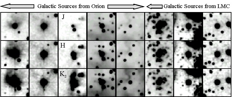Figure 18

Low Central Surface Brightness Galaxies

There are some galaxies whose central surface brightness is too low to be detected by the standard 2MASS procedure, but whose total integrated flux is significant (at least with respect to the 2MASS Level 1 specifications). These may include low surface brightness (LSB) galaxies, and dwarf or intrinsically small galaxies. We will refer to these sources with the generic moniker: low central surface brightness galaxies (LCSB). LCSB galaxies present a different challenge to GALWORKS than the typical "normal" galaxy 2MASS encounters. They are generally very faint (as measured in a standard aperture for "normal" galaxies) and they do not have well defined cores; see Figure 19 for examples of typical low central surface brightness galaxies found within 2MASS (Each image is 25´´ in width.) The integrated flux of the example sources range from J=15 to 15.6 and K_s=13.8 to 15.1 mag. The LSB galaxy nature of many of these sources is confirmed with deep optical images. There are some examples of galaxies observed to be low surface brightness in the near-infrared but normal in the optical-typically blue spiral galaxies.

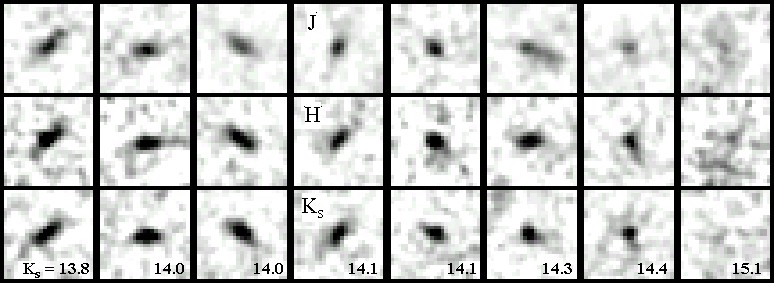Figure 19

The galaxy core is an important component for star-galaxy separation since many of the parametric measurements for star-galaxy separation are anchored to the core of the galaxy. The low central surface brightness detector (referred to as the LCSB processor) of GALWORKS is executed last in the chain of operations that comprise GALWORKS (see flowchart, Figure 2). The input to the LCSB processor is a fully cleaned Atlas image in each band, where stars brighter than some limit, typically K_s = 14.5 mag, and previously found extended sources have been entirely masked. The image is then blocked up (using three independent kernel sizes: 2×2, 4×4 and 8×8 pixels) and "boxcar" smoothed to increase the signal-to-noise ratio for large (but faint) objects normally hidden in the 1´´ correlated pixel noise. A block average is not the optimum method (as compared to a gaussian convolution, for example) but with pipeline runtime constraints it is a more satisfactory option.

The detection step consists of 3- threshold isolation of local peaks in the blocked-up cleaned images. Source detections are then parameterized (using the blocked and smoothed image) with the primary measurements being: signal-to-noise ratio of the peak pixel, radial extent (SH score), integrated signal-to-noise ratio, surface brightness, integrated flux, and SNR measurements using a J+H+K_s combined "super" image. The "super" image, in principle, provides the best median from which to find faint LSB galaxies given the effective increase in the signal-to-noise ratio. In practice, the "super" image only increases the SNR by approximately 30%-50% for normal (i.e., J-K_s ~ 1 mag) galaxy colors. Faint stars remaining in the cleaned image have a relatively low SNR since most of their light is confined to a few pixels that are averaged with blank sky in the blocking and boxcar-smoothing step. Galaxies, on the other hand, will add up since their light is distributed over a larger area.

The preliminary results for the LCSB processor demonstrate a reliability rate of about ~70 to 80% using a threshold on the "maximum" SNR (between 2×2, 4×4 and 8×8 blockings) of the "super" image. The major contaminants are faint stars and diffuse emission associated with bright stars. However, if a meteor streak (or other transient phenomenon) is present in the Atlas image(s), then numerous false sources are picked up as LSB galaxies.

We are still learning how to improve the reliability of sources coming from the LCSB detector. It is important to note that these sources are nearly always fainter than the Level 1 specifications (K_s > 13.5, J > 15 mag) which means that there are currently no requirements on the incompleteness and reliability. We do not anticipate significant completeness failure for LSB galaxies brighter than K_s ~ 13.5 mag. The fainter LSBs, however, will have to be detected and processed with the LCSB processor described here and released in a future special catalog. Enhancements of the algorithm described here are being studied, in particular, the multi-color "² image" technique described in Szalay et al. (1999, AJ, 117, 68) may prove to be a more robust and reliable technique at finding LCSB galaxies in the 2MASS database. Further information and some early science results with 2MASS LSB galaxies can be found in Jarrett (1998, in The Impact of Near-Infrared Sky Surveys on Galactic and Extragalactic Astronomy, p. 239) and Schneider et al. (1998, in The Impact of Large Scale Near-IR Sky Surveys, p. 187).

ix.Source Extraction

Sources that pass the star-galaxy discrimination tests and have an integrated flux brighter than the mag limits: J= 15.5, H = 14.8, K_s = 14.3 mag (MINUS the confusion noise for high source density fields), are extracted to the 2MASS extended source database. In addition to the parameters described in previous subsections, the source information includes various flags indicating stellar contamination, cross-identification (with previously catalogued large galaxies derived from the NASA Extragalactic Database) and processing status. A list of the "standard" extended source parameters can be found in the Extended Source Catalog Record Format table.

For each extended source, a small "postage stamp" image is clipped from the larger background-subtracted Atlas image. The stamp images are stored in J, H and K_s fits-format data cube files (see Appendix D for an example of a header). The image size is constrained by the final Kron or isophotal radius, with a minimum diameter of 21´´ and a maximum diameter of 101´´. The dynamic image size reflects the practical limitation of the finite storage capability of the 2MASS database. The stamp image headers provide all of the information needed to extract photometry, positions, etc., except the larger-area environment that was used to remove a local background (above) and evaluate contamination. For that reason the images include the background removed during the process described above. Since the background is already removed, it is a simple matter at computing source fluxes, they can be directly read (or summed within some aperture) from the images. The conversion of a 2MASS unit of flux ("dn" for data number, corresponding to the pixel value) is as follows:

(Eq. IV.5.8)

where f is the background-subtracted flux (in "dn" units), m₀ is the zero point calibration magnitude, and m is the desired (calibrated) magnitude. Consider the example given in Appendix B. Here the zero point calibration at K_s is 20.111 mag, while the image "noise" (RMS of the background) is 0.879 DN. It then follows that the 1- RMS in the K_s background is 20.250 mag/arcsec² (note that this RMS noise is applicable to size scales of ~2´´ × 2´´, corresponding to the effective resolution of the 2MASS survey).

d. 2MASS Extended Source Objects

The 2MASS extended source database is predominantly composed of galaxies, with a much smaller population of double and triple stars, at the 5 to 20% level depending on the stellar number density. Large-angular size Galactic objects, such as HII regions, stars with nebulosity, planetary nebulae, reflection nebulae, etc., are relatively rare and generally confined to the Galactic plane and a few other star formation sites around the Milky Way.

The extended source catalog is contaminated by a small 1-5% number of artifacts.

These false sources are generated in the vicinity of bright stars, by transient phenomenon, such as meteor streaks, and by infrared "airglow". Most artifacts associated with bright stars are easily identified within the 2MASS database using simple geometric removal algorithms, but which are not 100% effective. Meteor streaks are more difficult to identify using automated techniques, but in general their frequency is low. Airglow not only generates false detections (especially under severe conditions), but it also significantly affects the photometry of real sources. Examples of 2MASS galaxies and various kinds of artifacts are given below.

i. Galaxies

The 2MASS extended source database contains galaxies ranging in brightness from K_s=9 to 14 mag. This flux range is constrained by the sensitivity of the survey and size limitations fixed by the scale of the Atlas Image and the background removal process. Galaxies as large as 3 or 4´ in diameter may be processed (if they are located near the center of the Atlas image) but only the inner 2´ or so is examined in detail (c.f. Figure 9). For very large galaxies (>5´ in size), such as most of the Messier objects, the only processing is to extract pieces of Atlas images associated with the galaxy. At the faint end of the flux spectrum, it is difficult to determine the size of the galaxy due to the resolution of the survey, the elongation or asymmetry in the PSF, and the precise dither pattern. For the most part, we can reliably measure isophotal sizes down to a radius of 7´´.

In Figures 20, 21, and 22, a representative sample of galaxies from low stellar number density fields is shown with their K_s-band postage stamp images. The data come from scans passing through the Abell 3558, Hercules, & Abell 2065 clusters, as well as random non-cluster fields. A wide range in morphology, surface brightness and integrated flux comprise the sample. Figure 20 shows the brightest galaxies, ranging in total K_s-band flux from 9 to 13 mag. Each image is 60´´ × 60´´, demonstrating several morphological classes: elliptical (E), lenticular (S0, SA0), generic spiral (S), and complex irregular, including double nucleus, interacting and pre-merger systems. The next set of galaxies, Figure 21, represent the faint limit at which the extended source catalog is both reliable (>98%) and complete (>90%), with K_s ranging from 13 to 13.5 mag. The size of each image is 30´´ × 30´´. The final set of galaxies (Figure 22) represent the faintest galaxies resolved with 2MASS, with K_s ranging from 13.5 to 15 mag, corresponding to a SNR range between 4 and 8. Each image is 20´´ × 20´´ in width. The lowest surface brightness galaxies belong to this set, which are generally detected only in J-band due to the blue color of most LSB-type galaxies. For example, the last four galaxies in the set are detected in the J-band only.

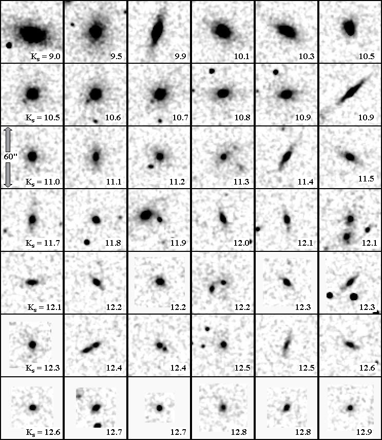
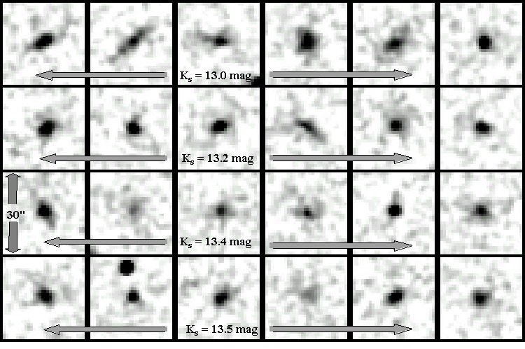
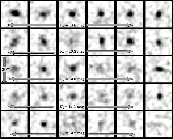Figure 20	Figure 21	Figure 22

When the source density is high, the confusion noise approaches the level of the atmospheric thermal background noise (see Appendix B). The probability of triple or multiple stars is significant and the ability to distinguish galaxies from multiple groupings of stars is strained. Nevertheless, a reliability of >80% is possible for most of the Galactic plane. Figure 23 gives examples of galaxies found in the Galactic plane, and for comparison, false extended sources (e.g., triple stars) found in the same areas. For the upper panels, the approximate Galactic coordinates are (240°, +4.5°), corresponding to a density of 4500 stars deg^-2 brighter than 14 mag, and a differential confusion noise equivalent of 0.7 mag in a 10´´ aperture (see Appendix B). The integrated K_s-band fluxes range from 11.8 to 13.8 mag. The estimated visual extinction is ~1 mag and the J-K_s reddening is ~0.15 mag. Closer to the Galactic center (Figure 23, middle panels), coordinates (12°, +5.0°), the density of stars is over 30,000 deg^-2, resulting in an equivalent differential K-band confusion noise of nearly 2 mags; yet, galaxies are still detected by 2MASS. The estimated visual extinction is now >2 mag and the J-K_s reddening is ~0.4 mag. Note the significant stellar contamination to the local environment of the galaxies. The integrated K_s-band flux ranges from 11.0 to 12.8 mag, indicative of confusion noise limits on the faint end detection spectrum. False detections are dominated by multiple stars (mostly triples and quadruples), a representative set is shown in the lower panels, Figure 23.

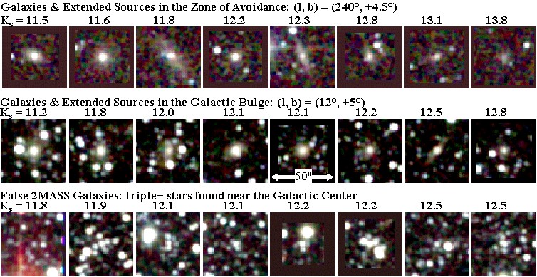Figure 23

ii. Galactic Extended Sources

Nebulosity associated with bright stars (e.g., H II regions, PNs, clusters) and with molecular clouds (reflection nebulae, YSOs) typically appear as very bright and large extended sources (Figure 24). Since these objects are primarily located deep in the Galactic plane, contamination by foreground stars is unavoidable.

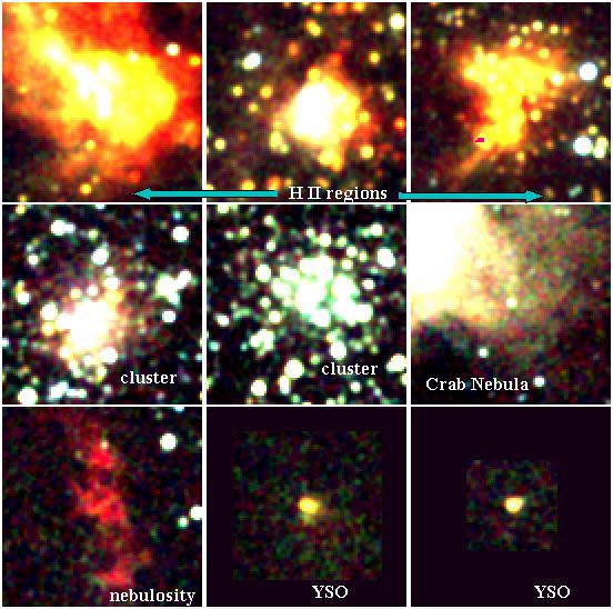Figure 24

iii. Bright Stars and Artifacts

Bright stars are a major nuisance to any image-based survey. Off-axis stray light can land just about anywhere on the focal plane, while dense concentrations of light (e.g., diffraction spikes) are distributed geometrically with respect to the optical axis. Features referred to as "glints" and "ghosts" are focused or semi-focused reflections of light that appear as slightly asymmetric point sources or flattened (low surface brightness) extended sources. Not only do bright 2MASS stars (K_s < 9 mag) produce diffraction spikes, halos, glints and ghosts, but the brightest stars (K_s < 5 mag) generate horizontal stripes that span the entire cross-scan (east-west axis) of the scan, or a total of 8.5´ in length. Worse, these stars are saturated, so we do not know their true integrated flux, making it difficult to anticipate the strength of their associated stripe, spike and persistence features (see below). Finally, bright stars induce another feature unique to infrared arrays: latent residual or persistence ghosts. The central core of a bright star leaves a residual signal after the array has been read out. The residual persists for several seconds (and for the brightest stars, many tens of seconds). Thus, a bright star will leave a "trail" of persistence ghosts as the telescope shifts in declination. All of these bright star artifacts, many of which strongly resemble galaxies, must be removed to meet the Level 1 requirements. The 2MASS pipeline and GALWORKS in particular, remove most of these artifacts (see below). During the catalog generation phase (i.e., after the pipeline reductions) we remove (or attempt to remove) the remaining artifacts that contaminate the database.

Halos, stripes and spikes have a well-determined geometry with respect to their progenitor, assuming that the integrated flux of the source is known. GALWORKS determines their extent by measuring their surface brightness, using limits based on the estimated total flux of the star and the expected confusion noise as traced by the stellar number density. Bright stars that saturate (K < 5 mag) may not have well determined stripe intensity, spike length or persistence coverage.

Diffraction spikes extend several arcminutes for very bright stars; see, for example, Figure 25, which shows a magnitude 4 star in a J-band Atlas image. Note the three horizontal stripes extended and flaring across the entire 8.5´ of the field, and the persistence ghosts trailing to the south of the bright star. An even more dramatic example of spikes, ghosts, halo and stripes is seen in Figure 26, which shows two adjacent J-band images with a K_s~ -1 mag star ( Pegasi) straddling the boundary. The vertical spikes extend well beyond the image boundaries, while the halo emission completely dominates both images. The persistence ghosts (trailing to the south of Peg) appear nearly as bright as field stars. The influence of Peg extends across scan boundaries as well, making it very difficult to identify and remove artifacts during the pipeline reductions. Hence, the database is significantly contaminated with false sources due to very bright stars such as Peg. Even in the post-processing stage, these sources present a major clean-up challenge: internal telescope reflections produce stripe/streak features extending over 1° in radius from the center of Peg (see Figure 27, right panel). In the vicinity of the brightest stars (K_s < 0 mag) in the infrared sky, it may not be possible to do an adequate artifact removal during the catalog generation. Fortunately, there are only a handful of these problematic stars spread throughout the sky.

Most meteor streaks have the unfortunate property of high surface brightness coupled with severe elongation-similar to large highly inclined spiral galaxies. Figure 27 demonstrates transient streaks in two different J-band Atlas images. Note the sharp boundaries for the bright streak and the episodic flaring for the fainter streak. The latter is, in fact, associated with Peg (Figure 26), discussed above. Meteor streaks are generally not identified in the pipeline reductions, resulting in false sources populating the extended source database. Instead, false sources due to "streaks" are removed during the catalog generation process: the one identifying feature is that usually multiple detections (in some cases several hundred sources) occur along the streak which can be identified with simple database queries and cleaned from the catalogs accordingly.

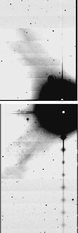
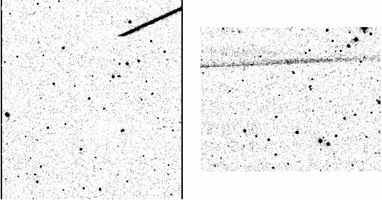Figure 25	Figure 26	Figure 27

Yet more artifacts are produced by bright to moderately bright stars on the edges of scans, as well as additional artifacts from meteor streaks and background gradients (for example, airglow "bumps" that are not removed). Figure 28 illustrates some of the kinds of artifacts found in the extended source database. The first two (reading left to right) are the result of a "ghost" or "glint", most prominent in J band, to the southwest of the 8 to 9 mag progenitor star. The third column shows a false detection due to a flared diffraction spike from a star on the edge of an Atlas image. The fourth and fifth columns are examples of faint stars or faint galaxies located on or within the boundary of a horizontal stripe or meteor streak. The final column is a faint star boosted in flux by background airglow (note the prominent H-band emission). Many of these artifacts are successfully removed during the catalog generation process. The airglow artifact is probably the most insidious class of false detection since it is so difficult to discriminate from real galaxies or real interstellar nebulosity. The only way to minimize their effect is to avoid data with significant airglow. H-only extended-source detections should be treated with caution.

We project that at the end of the 2MASS survey we will have detected over 2 million extended sources as faint as ~2 mJy. At 2.2µm, 2MASS will discover galaxies never seen before in the "Zone of Avoidance" where the obscuring effects of Galactic dust and gas limit traditional surveys.

Much of the algorithmic development was driven by the practical need for computational speed and efficiency (e.g., background removal and LCSB detection). As processing power increases over time, it will be possible to implement more sophisticated methods, including more robust methods for detection of low surface brightness galaxies. Moreover, we continue to build and expand the classification "training sets" to improve the performance of the decision tree classifier, while other methods (e.g., supervised neural nets) may also prove to be powerful star-galaxy discriminents. Future improvements will be focused upon reliability (star-galaxy-artifact discrimination) and completeness for SNR sources (e.g., LCSB galaxies).

In the future we will discuss in detail the completeness and reliability that can be expected for the release catalogs. The scientific content is assessed with analysis of the source counts and redshift distribution, size and orientation distributions, JHK_s colors, and coordinate position accuracy. Finally, we will discuss a method by which 2MASS extended sources may be used to identify and characterized galaxy clusters out to z ~ 0.2.

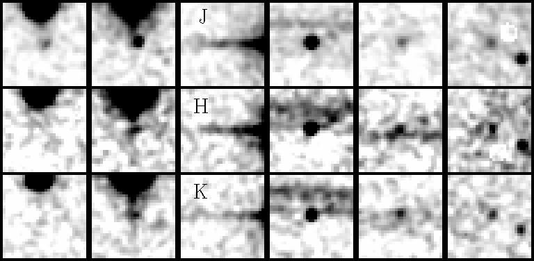Figure 28

 

Appendix A. Galaxy Photometry Error Tree

The fundamental limits to 2MASS galaxy photometry are set by the accuracy to which the background level can be determined, by the total signal-to-noise ratio in the aperture used to report the flux of a galaxy, and by the zero-point calibration used to adjust raw magnitudes onto a standard scale. Most of the time, the dominant error is the Poisson noise due to the background summed over the pixels used to make the photometric measurement and the uncertainty in the standard background removal itself (see above). However, a significant portion of the 2MASS data is affected by high-frequency background variation, which causes the photometric error to be larger for a small fraction of the galaxies. There are two sources for such background variations, one being atmospheric "airglow" and the other camera hardware related. In the near-infrared, the background levels generally fluctuate due to airglow emission, sometimes at very high spatial frequencies, particularly at 1.6 µm. In addition to airglow, 2MASS images include electronic ("pickup") noise that is correlated and can, at times, be comparable to the airglow component. Electronic pickup refers to image features that are not of astronomical origin, but instead are associated with the camera electronics. These features may manifest as periodic horizontal stripes or abrupt jumps in the background level. The impact is mostly felt in the galaxy photometry, where a systematic bias is introduced. This bias can be as large as 20% in some cases, but is more typically 3 to 7% (usually an overestimate of the galaxy flux). Examples of both forms of background enhancement are given in Figure 29.

i. Summary of Standard Photometric Error

For the usual case where the galaxy flux is negligible compared to the background flux, the measurement error in summing up the flux over n pixels in the Atlas image is

(Eq. IV.5.9)

where _pix is the measured pixel noise as measured using an entire Atlas image (512×1024 pixels). The factor of 1.7 accounts for the smoothing introduced in the Atlas image by the frame resampling and construction process, and the factor of 4 results from the correlation of the flux in 1´´ pixels, due to the 2´´ camera (raw frame).

GALWORKS also models and subtracts variations in the background using a polynomial fitting scheme described above. If the background variations are small on time scales of a few seconds, the fitting procedure is limited primarily by the effective RMS in the background sky noise, _pix. The fitting procedure usually can match the background over regions as small as ~2´ to 3´. Empirical tests indicate that the background fitting procedure is accurate to within 3 to 5% of the RMS pixel noise (in the absence of abrupt background structure coming from high-frequency airglow or electronic banding, which is usually the case for the 2.2µm images). Since errors in the background contribute systematically to all pixels in a galaxy smaller than 3´, this error contributes in proportion to the number of pixels n. The total photometric noise variance is the quadratic sum of these two terms

(Eq. IV.5.10)

It is clear that the first term dominates the total error except when the number of pixels within the aperture is very large, n > 10⁴ (corresponding to a circular radius > 40 to 50 pixels). This also assumes that background variation is well behaved. Most galaxies detected in 2MASS are small and faint, so the Poisson noise component (Eq. IV.5.9) should dominate the total photometric error. Consider for example a K_s=13 mag galaxy. The integrated flux is ~630 DN (or ~4.5 mJy) using a typical K_s zero point magnitude of 20.0 mag (relating the calibrated mag to the raw or "data number" flux; see Eq. IV.5.8). The typical size for a galaxy of this brightness is about 16´´ in diameter, corresponding to a circular aperture with ~200 pixels. The typical K_s background pixel noise is ~1 DN (or 20 mag per arcsec²). Using Eq. IV.5.10 and the integrated flux of the source, we compute a SNR of 12.6 to 12.8, where the Poisson component is 25 to 70 times larger than the background-fit uncertainty (i.e., the noise contribution from the background fitting procedure is very small, only 1 to 4% of the total photometric noise). For larger (and hence less common) galaxies, the size of the galaxy must be greater then ~35´´ in diameter for the uncertainty in the background fit to become appreciable (>10% of the total).

If the background variation requires a higher-power polynomial than a cubic, then the error in the background will no longer be determined by the pixel noise. Instead, the background error will result from the residual error after a cubic polynomial is fit. This will be the case for severe airglow variation, which can modulate on high spatial frequency scales (see left panel, Figure 29), and from correlated "electronic" noise (see right panel, Figure 29). Both conditions can easily boost the total photometric noise by >50%. Unfortunately, the 2MASS data reduction pipeline is not adequately designed to quantify these severe background variations; and indeed, high-frequency background variations may go undetected from scan to scan. We are exploring methods at which detection and correction of severe 'airglow features" may be possible, particularly for the H-band data. Fortunately, the hardware-induce background variations are diminishing with maturity of the 2MASS survey.

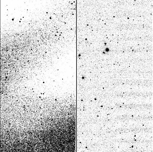Figure 29

ii. Adaptive Aperture Errors

Adaptive apertures (i.e., Kron and isophotal) come in two different shapes: circular and elliptical. Circular apertures are fully described by the radius, fit to the desired isophote. Elliptical apertures are described by three parameters, radius (semi-major axis), axis ratio and position angle, fit to the desired isophote. The fitting procedures introduce additional uncertainties. Here we assume the uncertainty due to the position of the isophote is negligible.

For the circular case, the radius has an error that is driven by background noise and contamination (i.e., stars near or within the isophote). Errors in the determination of that radius dominate the photometric error tree. Consider the typical case of a galaxy with an exponential profile. The integral flux over a circular aperture is

(Eq. IV.5.11)

where r is the aperture radius divided by the radial scale length of the galaxy profile. The flux error caused by the error in radius determination is

(Eq. IV.5.12)

For a disk scale length of 2´´, and typical isophotal 20 mag arcsec^-2 aperture radii of 6 to 8´´, the flux error ranges between 0.08 and 0.19 × r. The typical width or uncertainty of the circular isophote is about 1´´, so r=0.5 and the resultant flux error ranges between 4-9%. The Poisson photon noise in an aperture of this size gives typical flux errors of ~5-7%, and hence the radius uncertainty is comparable to the photon-noise contribution for this K_s~13 mag spiral galaxy case.

For elliptical aperture photometry, in addition to the radial uncertainty, two additional parameters (axial ratio and position angle) add to the total error budget. However, there is some positive compensation due to the fact that the orientation of galaxies is elliptically shaped; thus, optimal elliptical apertures minimize the background noise contribution and systematics due to measurement error in the background itself (above). Analysis of the 2MASS extended source database reveals that for 2MASS galaxies brighter than ~13 mag, the elliptical aperture photometry gives the most precise measurement of the galaxy flux. Note however that the elliptical aperture is vulnerable to contamination, especially in high source density regions, which makes it susceptible to large uncertainties if the ellipse parameters are inaccurate. For faint galaxies, the PSF shape and image resolution generally favor a circular aperture to that of an ellipse because the galaxies are so small that the ellipse parameters are highly uncertain.

Appendix B. Stellar Number Density and Confusion Noise

As the surface density of stars exponentially increases near the disk of the Galaxy, the probability of source contamination increases accordingly. Likewise, near the Galactic plane, faint undetected stars significantly increase the mean "noise" amplitude in the "background" sky. Both surface density affects limit the source detection or completeness, and overall reliability. Confusion arises from the appearance of an interloping star within close proximity to the "beam" or point spread function pattern that induces a significant flux bias (or "deflection") from the non-contaminated flux due to the intended source (in our case, galaxy) near the beam center. A convenient gauge for the severity of contamination or level of source confusion, is the confusion "noise". In more practical form, the confusion noise represents the change in surface brightness (i.e., sensitivity limit) relative to the Galactic pole (where the confusion noise is negligible), expressed in magnitude units. The confusion noise is directly related to the stellar number density. In the 2MASS database the stellar number density is referred to as the "density", representing the base-10 log of the cumulative number of stars per deg² brighter than K_s=14 mag (see also Table 1).

As the confusion noise becomes appreciable, it is one of the primary limits on galaxy detection and reliability. Moreover, confusion decreases the accuracy of both flux and position estimation. It is therefore important to understand the confusion noise in terms of the ability to detect isolated sources and in terms of identification of real extended sources, both of which require threshold adjustment with confusion noise level.

i. Estimation of Confusion Noise

To estimate the additional component of "confusion" noise, we adopt the methodology of Hacking (1987, PhDT) and Hacking & Houck (1987, ApJS, 63, 311). The idea is to integrate the expected number of sources (with some flux distribution) within the 2MASS effective beam, , where represents the effective radius of the point spread function (typically ~2´´). We may approximate the stellar flux distribution with a power law of index ,

(Eq. IV.5.13)

where N is the integrated stellar number density (in deg²) at flux f (in mJy). The aggregate variance due to background sources in the beam, derived from f, d and the differential stellar number density, is then

(Eq. IV.5.14)

where D_c represents the outlier or "deflection" cutoff point (in n- units; i.e., the detection threshold). The source density index is approximately equal to unity (more precisely ~0.85 for high latitude fields) as derived from the log-log slope of the N vs. K_s cumulative star count curve, ~0.35 for the NGP and slightly steeper at higher densities (Jarrett 1992, PhDT). Letting , we may express the confusion noise as a function of the stellar number density, N(f_lim), at the limiting flux, f_lim, and the deflection cutoff, q,

(Eq. IV.5.15)

Appropriate values for 2MASS K_s-band data are the following: = 0.9, = 13.6 arcsec² (4´´ beam), f_lim = 1.8 mJy (corresponding to K_s=14 mag), and q between 3 and 5; the confusion noise has units of mJy.

The confusion noise adds in quadrature to the already present background noise, , raising the overall noise and surface brightness of the background light. We desire to express the change in the background surface brightness due to confusion noise as a function of the stellar number density. We can turn the confusion noise into a surface brightness by dividing by . For the background sky noise we adopt a value of 20.0 mag/pixel (typical for 2MASS 2.2 µm images). To convert the sky noise per pixel to an equivalent surface brightness within the PSF beam, we need to divide by to account for the noise limit after averaging over a 4´´ diameter. Accordingly, we arrive at a sky noise surface brightness of 21.6 mag/arcsec², representing the value at the north Galactic pole (NGP), which is negligibly affected by confusion from stars. The confusion noise (in mag units) is relative to the NGP sky surface brightness noise (in a 4´´ diameter beam). The K_s-band confusion noise as a function of the total integrated stellar number density (f_lim < 1.8 mJy, or K_s < 14 mag) is plotted in Figure 30, described below, assuming a beam size of 4´´, = 0.9 and q between 3 and 5.

ii. Confusion Noise, Stellar Density and Galactic Coordinates

For relatively moderate flux ranges (e.g., V < 18; K_s < 14), basic three-component models of the Galactic stellar distribution adequately describe the number density of dwarf and giant stars comprising "disk" and "spheroid" populations (Elias 1978, ApJ, 224, 453; Bahcall & Soneira 1980, ApJS, 44, 73; Garwood & Jones 1987, PASP, 99, 453). Here we employ a near-infrared modified variation on the Bahcall & Soneira model, which predicts the stellar number density with ~90% accuracy for most of the sky (|b| > 30°) and K_s < 14 mag, and performs adequately (~80%) for the Galactic plane where patchy extinction ultimately limits the utility of these simple models. The star-count model predicts the stellar number density as a function of the Galactic coordinates, which can then be used to calculate the approximate confusion noise.

A plot of the stellar number density as a function of the Galactic latitude along two separate longitudes (50° and 130°) is shown in Figure 30. The vertical dotted lines represent the thresholds for what is deemed low stellar number density (<10^3.1 stars deg^-2), moderate density (<10^3.6 stars deg^-2), and high density (>10^3.6 stars deg^-2). The limit on high density is partly driven by the relative density of triple stars vs. double or single stars. As triple+ stars become appreciable, the ability to distinguish real galaxies from close groupings of stars is greatly diminished. Finally, the confusion noise (mag) appropriate to the stellar number density is plotted in Figure 30 (denoted with a cross-hatching, showing the detection threshold range in q between 3 and 5), with the confusion noise axis located at the right of the plot. Here the confusion noise (in mag units) is relative to the equivalent sky background surface brightness (1- detection limit) measured at high galactic latitudes (i.e., NGP), equal to 0.0016 mJy (in a 4´´ circular diameter beam) or 21.6 mag at 2.2 µm. This relative confusion noise is called the "differential" confusion noise above.

Figure 30

Appendix C. Extended Source Catalog Parameters

The 2MASS Extended Source database contains over 400 parameters per source, most of which are related to photometry. The public-accessible catalogs are derived from this database. In Table 1 a condensed list is given of the most important parameters in the catalogs. The list includes positions, ellipse-shape geometry, photometry, surface brightness, star-galaxy discrimination scores, symmetry, and "probability of extendedness" (see above). The parameter name represents the actual designation used in the catalogs and database.

For galaxy photometry and colors, we recommend the fiducial K_s-band 20 mag arcsec^-2 ellipse-aperture measurements only for brighter galaxies. However, for smaller galaxies (comprising most of the catalog) the fixed R=7´´ circular-aperture values are the most robust flux measures; see Table 1. For each flux measure there is an associated confusion flag, where a non-zero value indicates stellar contamination.

Appendix D. 2MASS Extended Source Data Cube FITS Header

For each extended source, a small "postage stamp" image is extracted from the J, H and K_s Atlas images, with the background removed from each band (see above). The image size is scaled by the final Kron or isophotal diameter, with a minimum diameter of 21´´ and a maximum diameter of 101´´. The multi-band information is stored in a FITS cube, with the J image occupying the first plane, H in the second plane and K_s in the third plane. The header (see example below) contains the following information: catalog identification (e.g., NED name, if any), observation date and time, equatorial coordinate information, median background level before removal and the background "noise", PSF "shape" value (representing the radial extent of the PSF at the time of the observation; see above and Eqs. IV.5.2 and IV.5.3), zero point calibration magnitudes and the airmass. The background and "noise" values are given in "dn" (or data number) units. See Eq. IV.5.8 (above) for a conversion of "dn" flux units to calibrated magnitudes.

bitpix = -32
NAXIS = 3
NAXIS1 = 101
NAXIS2 = 101
NAXIS3 = 3
BSCALE = 1.
BZERO = 0.
GID = '000228 ' / 2MASS ID #
NNAME = 'NGC_4551' / NED Cat Name
ScanNo = '065 ' / Scan Number
CoaddNo = '256 ' / Coadd Number
ORDate = '980115n ' / Observation Ref Date (yymmdd)
UT_DATE = '980115 ' / UT Date of Frame (IC) (yymmdd)
UT = '11:04:07.23' / Time of Frame (IC) (sxgsml)
EQUINOX = 2000. / Equinox
CTYPE1 = 'RA---SIN' / Orthographic Projection
CTYPE2 = 'DEC---SIN' / Orthographic Projection
CRPIX1 = 51.
CRPIX2 = 51.
CRVAL1 = 188.9082336 / RA at Frame Center, J2000 (deg)
CRVAL2 = 12.26402664 / Dec at Frame Center, J2000 (deg)
CROTA2 = -0.009442620911 / Image Twist E of N, J2000 (deg)
CDELT1 = -0.0002777777845 / Axis 1 Pixel Size (degs)
CDELT2 = 0.0002777777845 / Axis 2 Pixel Size (degs)
RA = 188.9082336 / RA at Frame Center, J2000 (deg)
DEC = 12.26402664 / Dec at Frame Center, J2000 (deg)
JSKYVAL = 115.1816559 / GALWORKS J Sky Measurement
JSKYSIG = 0.5367393494 / GALWORKS J Noise Measurement
HSKYVAL = 492.6220398 / GALWORKS H Sky Measurement
HSKYSIG = 1.073829651 / GALWORKS H Noise Measurement
KSKYVAL = 277.62323 / GALWORKS K Sky Measurement
KSKYSIG = 0.8794555664 / GALWORKS K Noise Measurement
CALID = ' CALIBRATED' / Calibration ID
JSEESH = 0.9869999886 / Seeing J shape parameter
HSEESH = 0.9620000124 / Seeing H shape parameter
KSEESH = 0.9380000234 / Seeing K shape parameter
JMAGZP = 21.1258 / Calibrated J zero point from CALMAN
HMAGZP = 20.7288 / Calibrated H zero point from CALMAN
KMAGZP = 20.1106 / Calibrated K zero point from CALMAN
AMASS_FC= 1.118124962 / Airmass (aprox) at this position
ORIGIN = '2MASS ' / 2MASS Survey Camera

[Last Updated: 2000 Feb 18; by T. Jarrett, T. Chester, S. Schneider, S. Van Dyk, & R. Cutri]

---

Previous page. Next page.
Return to Explanatory Supplement TOC Page.