VI. Analysis of the 2MASS Second Incremental Release Catalogs
6. PSC Reference Field Characteristics
a. Global Statistics for the PSC
Introduction
These statistics are based on 12,800 queries to the local database for equal area tiles. The statistics are as follows. We made a cut at signal-to-noise ratio (S/N) = 30. For each of the high and low S/N subsamples we computed at each band:
- Means of quoted
 and
and  2
2
- Standard deviation about mean for these
- Rank value such that 1% are below value ( and 2) [Not shown]
- Rank value such that 1% are above value ( and 2)
- Number in bin (divide by 3.22 to get number per square degree)
The figures below are Aitoff projections of isovalue maps in galactic coordinates for each of these quantities.
Details
The coordinate space was divided into 160 bins in galactic longitude and 80 bins in x=cos(colatitude). The distribution in each quantity was binned and summed to get the cumulative distribution function along with the sample statistics. The rendering was done using the VTK package. The data blanking facility was not working, so cells with no data are shown as red. There are some edge artifacts where the bins in galactic coordinates very poorly sample the Second Incremental Data Release areas.
Number density of sources
Figures 1 and 2 show true number density, not number per bin, with linear and logarithmic contour levels, respectively. There are no surprises here. The gaps in coverage give the illusion of structure in the plane.

|

|
| Figure 1 | Figure 2 |
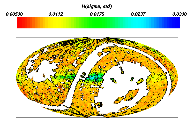
Quoted Error
Shown in Figures
3,
4, and
5, and
15,
16, and
17
are the mean plots
for each 2MASS band for high S/N sources
and low S/N sources, respectively.
Overall, the error appears very uniform north to south.
The error is better in the south than in the north at Ks.
This is subtle and only obvious for the high S/N sources.
The northern error is more variable than the south.
There is a large error feature in the Galactic plane at H
(galactic longitude l of about 245°). We are not sure if this is
real, or some sort of numerical artifact.
For low S/N sources, the trend reverses, which may be
an artifact of source density confusion in the plane; only high S/N
sources are recovered.
Shown in Figures
6,
7, and
8, and
18,
19, and
20
are the standard deviation plots.
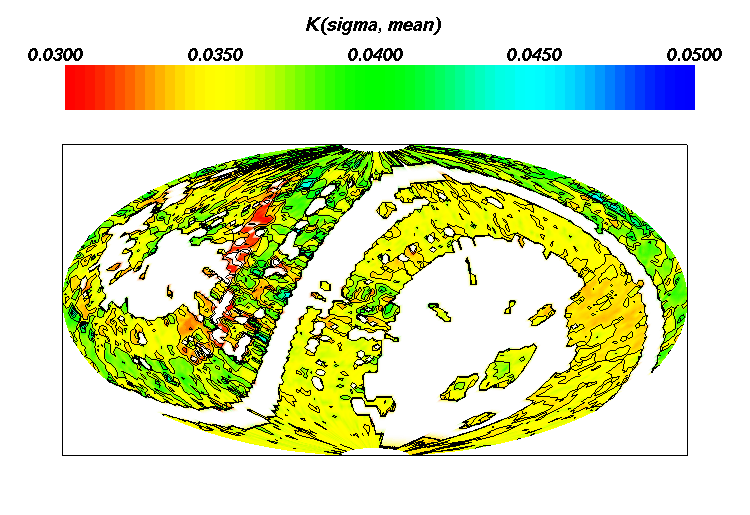
The Galactic plane is a smaller variance about the mean at J and
larger at Ks (again, H is distorted by the big error bump).
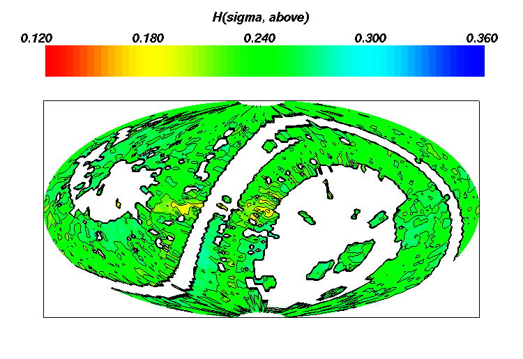
Shown in Figures
9,
10, and
11, and
21,
22, and
23
are the 1% tail value.
These show, not surprisingly, that the error values in
the Galactic plane have a heavy tail (again, H is distorted by the high error
feature, or analysis bug)
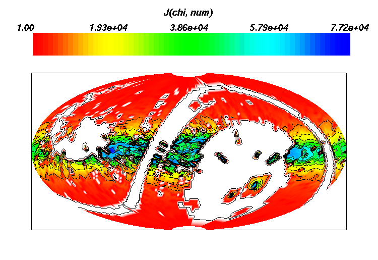
Shown in Figures
12,
13, and
14, and
24,
25, and
26
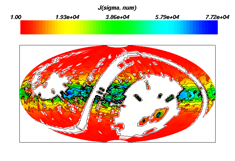
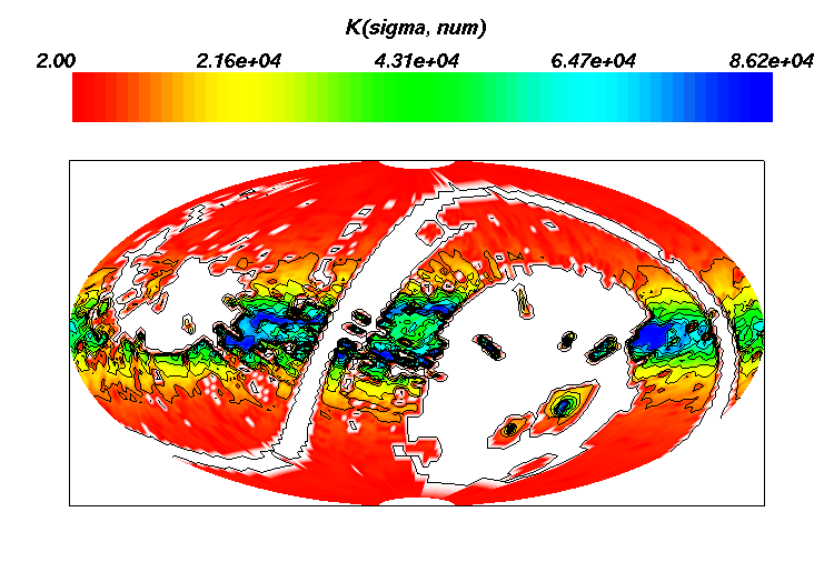
are the number per bin value.
At low S/N, one sees the lower recovery fraction in the plane of the
Galactic disk.
| High signal-to-noise ratio data (S/N>30) | ||
| J | H | Ks |
 |
 |
 |
| Figure 3 | Figure 4 | Figure 5 |
 |
 |
 |
| Figure 6 | Figure 7 | Figure 8 |
 |
 |
 |
| Figure 9 | Figure 10 | Figure 11 |
 |
 |
 |
| Figure 12 | Figure 13 | Figure 14 |
| Low signal-to-noise ratio data (S/N<30) | ||
| J | H | Ks |
 |
 |
 |
| Figure 15 | Figure 16 | Figure 17 |
 |
 |
 |
| Figure 18 | Figure 19 | Figure 20 |
 |
 |
 |
| Figure 21 | Figure 22 | Figure 23 |
 |
 |
 |
| Figure 24 | Figure 25 | Figure 26 |
The tables below show the "Top 10" fields ranked by mean quoted error. All but the top few in some cases are nominal and are included to provide a baseline. The field with galactic longitude and latitude 254.25°< l <254.5° and -1.4° < b <0° is large at both J and Ks, but only contains 7 sources.
| High S/N at J | Low S/N at J | ||||||||
| l1(°) | l2(°) | b1(°) | b2(°) | j_sigma_hi_mean | l1(°) | l2(°) | b1(°) | b2(°) | j_sigma_lo_mean | 254.25 | 256.5 | -1.43254 | 0 | 0.087 | 184.5 | 186.75 | -40.5416 | -38.6822 | 0.143 | 290.25 | 292.5 | -44.427 | -42.4542 | 0.05 | 348.75 | 351 | -50.805 | -48.5904 | 0.136 | 267.75 | 270 | 67.6684 | 71.8051 | 0.046 | 58.5 | 60.75 | -67.6684 | -64.1581 | 0.136 | 42.75 | 45 | 1.43254 | 2.86598 | 0.0447592 | 240.75 | 243 | -31.6682 | -30 | 0.135 | 355.5 | 357.75 | 1.43254 | 2.86598 | 0.0445452 | 51.75 | 54 | 26.7437 | 28.3594 | 0.134 | 45 | 47.25 | 0 | 1.43254 | 0.0439315 | 254.25 | 256.5 | -1.43254 | 0 | 0.1224 | 114.75 | 117 | -53.1301 | -50.805 | 0.0433333 | 36 | 38.25 | 36.8699 | 38.6822 | 0.118167 | 51.75 | 54 | 26.7437 | 28.3594 | 0.043 | 101.25 | 103.5 | -20.4873 | -18.9656 | 0.1145 | 330.75 | 333 | -2.86598 | -1.43254 | 0.0429486 | 141.75 | 144 | 61.045 | 64.1581 | 0.1135 | 135 | 137.25 | 0 | 1.43254 | 0.0420386 | 137.25 | 139.5 | 64.1581 | 67.6684 | 0.112773 |
| High S/N at H | Low S/N at H | ||||||||
| l1(°) | l2(°) | b1(°) | b2(°) | h_sigma_hi_mean | l1(°) | l2(°) | b1(°) | b2(°) | h_sigma_lo_mean | 254.25 | 256.5 | -1.43254 | 0 | 0.194 | 348.75 | 351 | -50.805 | -48.5904 | 0.209 | 42.75 | 45 | 1.43254 | 2.86598 | 0.0552654 | 254.25 | 256.5 | -1.43254 | 0 | 0.1718 | 252 | 254.25 | 64.1581 | 67.6684 | 0.053 | 308.25 | 310.5 | -44.427 | -42.4542 | 0.153 | 45 | 47.25 | 0 | 1.43254 | 0.0509786 | 36 | 38.25 | 36.8699 | 38.6822 | 0.150583 | 4.5 | 6.75 | 58.2117 | 61.045 | 0.0509545 | 294.75 | 297 | -53.1301 | -50.805 | 0.146 | 51.75 | 54 | 26.7437 | 28.3594 | 0.0495 | 153 | 155.25 | 36.8699 | 38.6822 | 0.142429 | 191.25 | 193.5 | 36.8699 | 38.6822 | 0.0492357 | 306 | 308.25 | 53.1301 | 55.5885 | 0.141667 | 58.5 | 60.75 | -22.0243 | -20.4873 | 0.0490068 | 159.75 | 162 | 17.4576 | 18.9656 | 0.1416 | 60.75 | 63 | -18.9656 | -17.4576 | 0.0483095 | 353.25 | 355.5 | 42.4542 | 44.427 | 0.138909 | 67.5 | 69.75 | 15.962 | 17.4576 | 0.048191 | 150.75 | 153 | 11.537 | 13.0029 | 0.133948 |
| High S/N at Ks | Low S/N at Ks | ||||||||
| l1(°) | l2(°) | b1(°) | b2(°) | k_sigma_hi_mean | l1(°) | l2(°) | b1(°) | b2(°) | k_sigma_lo_mean | 153 | 155.25 | 36.8699 | 38.6822 | 0.049 | 290.25 | 292.5 | 30 | 31.6682 | 0.197333 | 193.5 | 195.75 | 40.5416 | 42.4542 | 0.0478305 | 58.5 | 60.75 | -67.6684 | -64.1581 | 0.170333 | 45 | 47.25 | 0 | 1.43254 | 0.0471634 | 342 | 344.25 | 46.4688 | 48.5904 | 0.16 | 45 | 47.25 | 33.367 | 35.0996 | 0.046 | 159.75 | 162 | 17.4576 | 18.9656 | 0.1554 | 42.75 | 45 | 1.43254 | 2.86598 | 0.0459062 | 112.5 | 114.75 | 30 | 31.6682 | 0.155286 | 171 | 173.25 | -5.73917 | -4.30122 | 0.0458865 | 36 | 38.25 | 36.8699 | 38.6822 | 0.139917 | 47.25 | 49.5 | 35.0996 | 36.8699 | 0.045579 | 87.75 | 90 | 44.427 | 46.4688 | 0.138476 | 45 | 47.25 | 35.0996 | 36.8699 | 0.0453898 | 119.25 | 121.5 | -53.1301 | -50.805 | 0.138167 | 189 | 191.25 | 40.5416 | 42.4542 | 0.0453732 | 308.25 | 310.5 | -44.427 | -42.4542 | 0.1374 | 60.75 | 63 | -20.4873 | -18.9656 | 0.0451757 | 108 | 110.25 | -25.1507 | -23.5782 | 0.134939 |
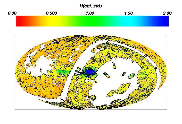
Chi-Square 2
Shown in Figures
27,
28, and
29, and
39,
40, and
41
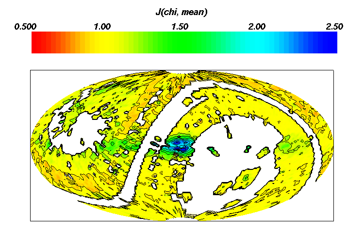
are the mean 2 plots
for each 2MASS band for high S/N sources
and low S/N sources, respectively, which are consistent
with a value of 1 in all bands, except for the higher values
realized in the Galactic plane.
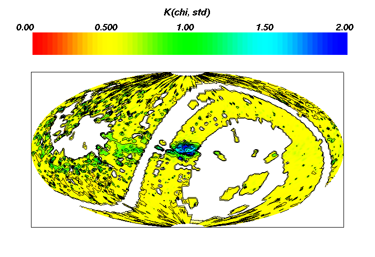
Shown in Figures
30,
31, and
32, and
42,
43, and
44
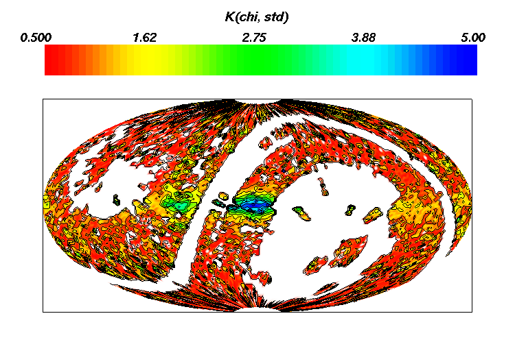
are the standard deviation 2
plots. We see larger variance in the Galactic plane and for
Ks in the north. In general, the large variance
regions indicate errors not included in the extraction error model.
Shown in Figures
33,
34, and
35, and
45,
46, and
47
are the 1% tail 2 value
plots. There is a slightly odd, unexplained feature in the Galactic plane.
Shown in Figures
36,
37, and
38, and
48,
49, and
50
are the number per bin 2 value.
There is a similar dip at low S/N near the Galactic plane, as seen
in the quoted error plots above.
| High signal-to-noise ratio data (S/N>30) | ||
| J | H | Ks |
 |
 |
 |
| Figure 27 | Figure 28 | Figure 29 |
 |
 |
 |
| Figure 30 | Figure 31 | Figure 32 |
 |
 |
 |
| Figure 33 | Figure 34 | Figure 35 |
 |
 |
 |
| Figure 36 | Figure 37 | Figure 38 |
| Low signal-to-noise ratio data (S/N<30) | ||
| J | H | Ks |
 |
 |
 |
| Figure 39 | Figure 40 | Figure 41 |
 |
 |
 |
| Figure 42 | Figure 43 | Figure 44 |
 |
 |
 |
| Figure 45 | Figure 46 | Figure 47 |
 |
 |
 |
| Figure 48 | Figure 49 | Figure 50 |
Signal-to-Noise Ratio
Shown in Figures 51, 52, and 53, and are plots for each 2MASS band for sources with S/N > 7. Shown in Figures 54, 55, and 56, and are plots for each 2MASS band for sources with S/N > 10. Shown in Figures 57, 58, and 59, and are plots for each 2MASS band for sources with S/N > 20. The effect of differing sensitivity between the bands is clear: a small fraction of sources below S/N=7 at J, larger number at H, and even larger at Ks. At Ks, the Galactic plane is clearly "avoided" at these small S/N. Some trends of north vs. south are evident at Ks, especially at S/N < 7. There is a hint of this at S/N < 10 and S/N< 20 as well, but only at Ks.
Shown in Figures 60, 61, and 62, and are plots for each 2MASS band for sources with S/N > 30. We were a bit surprised that 93% of the sources have S/N below 30 at Ks!
| J | H | Ks | |
| SNR < 7 |  |
 |
 |
| Figure 51 | Figure 52 | Figure 53 | |
| SNR < 10 |  |
 |
 |
| Figure 54 | Figure 55 | Figure 56 | |
| SNR < 20 |  |
 |
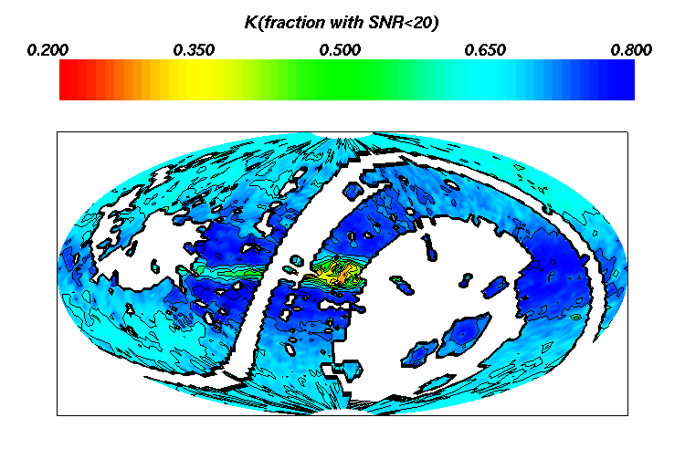 |
| Figure 57 | Figure 58 | Figure 59 | |
| SNR < 30 |  |
 |
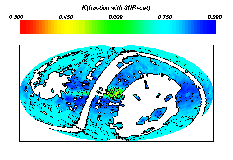 |
| Figure 60 | Figure 61 | Figure 62 |
Global Color Statistics
The goal of this analysis is to look for color changes over the entire sky.
This can be accomplished through a narrow cut near the peak in
the color-color plane and then compute the statistics in the distribution
of J-Ks. Figure 63
shows the color-color (Hess) diagram with color cut 0.30
In Figures 65,
66, and
67 are shown the mean in,
the standard deviation in, and the number, respectively, of high S/N sources
for J-Ks.
In Figures 68,
69, and
70 are shown the 20%, 50%, and 80%
fraction, respectively, of high S/N sources for J-Ks.
In Figures 71,
72, and
73 are shown the mean, 50% fraction,
and 60% enclosed width, respectively, of low S/N sources for J-Ks.
We have more closely examined the H-band behavior on the color
statistics in Figures 74-97. We compare the J-Ks maps
with the H-Ks
maps, to show the H-band behavior relative to J and Ks. We
also show the pattern orthogonal to J-Ks on the standard
two-color plane (J-H, H-Ks), which should be approximately
reddening independent. At the spatial scale shown in the figures, there
is only weak evidence of slightly poorer H-band stability. The
"reddening-free" flux ratio shows a weak dependence at higher galactic
latitude. There is clearly a smaller range in this variable towards the
plane, but it will be difficult to deconvolve the S/N and sensitivity
selection effects from both reddening and population differences.
Summary
Overall, the data appear to meet the Level 1
specifications on average.
Regions with sources with anomalously large error are given in the
tables in the "Quoted Errors" subsection, above.
The top offender has only seven sources; excluding this one,
there are no terrible fields.
Ks-band had noticeably higher excursions in the north in
quoted error for high S/N sources (excluding the plane).
[Last Updated: 1999 Dec 27 by M. Weinberg.
Modified 2000 Sep 13 by S. Van Dyk.]


Figure 63 Figure 64


Figure 65 Figure 66 Figure 67


Figure 68 Figure 69 Figure 70

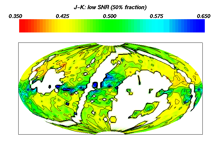
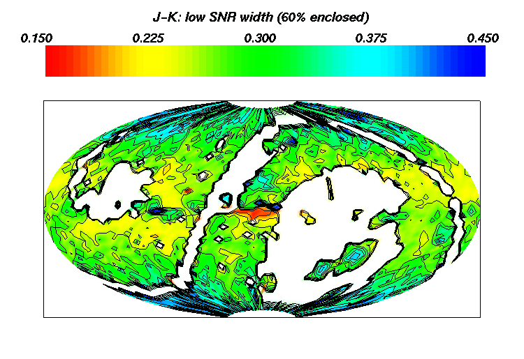
Figure 71 Figure 72 Figure 73
J-Ks
H-Ks
(J-H)-(H-Ks)
High SNR: mean


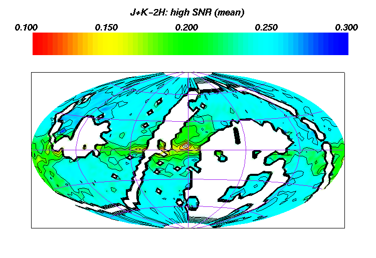
Figure 74 Figure 75 Figure 76
High SNR: std. dev.


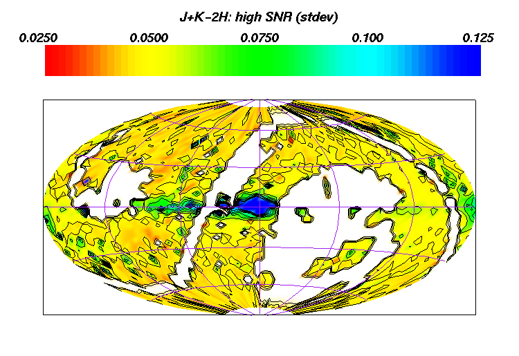
Figure 77 Figure 78 Figure 79
High SNR: fraction 50%


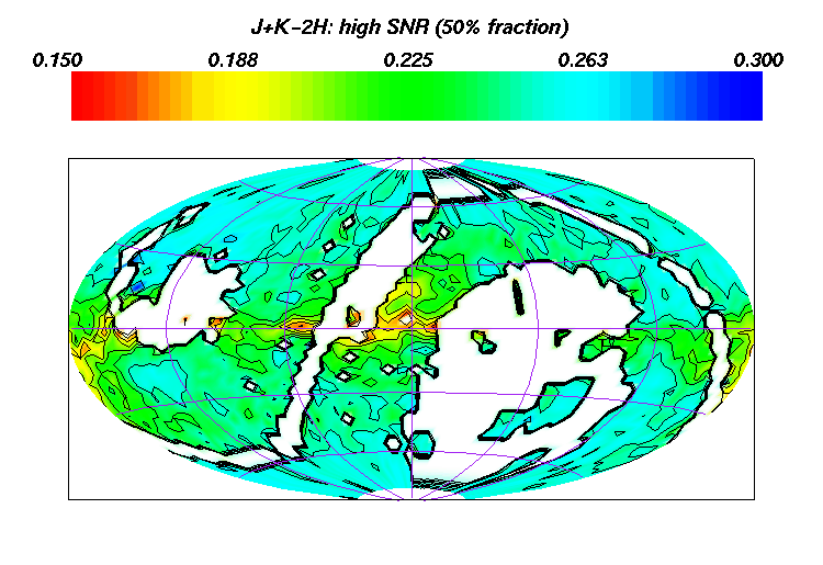
Figure 80 Figure 81 Figure 82
High SNR: width 60%
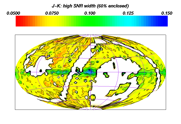


Figure 83 Figure 84 Figure 85
Low SNR: mean


Figure 86 Figure 87 Figure 88
Low SNR: std. dev.


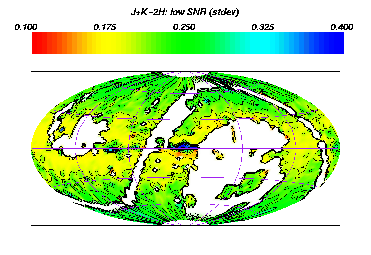
Figure 89 Figure 90 Figure 91
Low SNR: fraction 50%
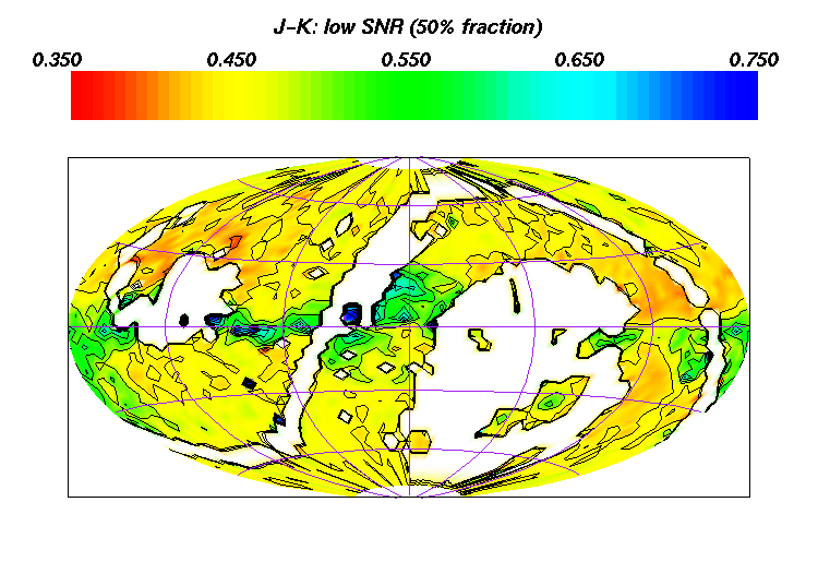


Figure 92 Figure 93 Figure 94
Low SNR: width 60%


Figure 95 Figure 96 Figure 97
Return to Section VI.6.