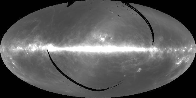
2MASS All Sky Images
| Image | Linear stretch | Log stretch | Number of stars | Selection Criteria | |||||||||
|---|---|---|---|---|---|---|---|---|---|---|---|---|---|
Star count maps | |||||||||||||
| Level 1 specs | J H K | J H K |
|
|
|||||||||
| All magnitudes | J H K | J H K |
|
|
|||||||||
| "Bright" stars (mag <= 11) |
J H K | J H K |
|
|
|||||||||
| Single band detections (no mag limits) |
J H K | J H K |
|
|
|||||||||
| Single band detections (J<=15.8, K<=14.3) |
J H K | J H K |
|
|
|||||||||
Color maps | |||||||||||||
| Level 1 specs |
J-K
J-H
H-K
100um |
J-K
J-H
H-K
100um |
|
|
|||||||||
Astrometric uncertainties | |||||||||||||
| Major axis | J H K |
|
|
||||||||||
| Minor axis | J H K |
|
|
||||||||||
Notes
Single-band detections
- While inspecting the single band detection images, I found a few
regions of enhanced J-only and K-only detections. These are difficult
to see on the gif images above, but are clearly visible on the fits
images.
One such region is at (ra=69.2, dec=-62.1).
To investigate this further, I downloaded from gator sources within a 1 deg radius of this position that had a cc_flg of '000'. Figure 1a shows the spatial plot of the single band detections, and Figure 1b shows a similar spatial plot but for sources brighter than the Level 1 specs. These plots clearly show that these single band detections are artifacts along the diffraction spikes of a bright star. The brightest star in this field has a magnitude of (J=-2.652, H=-3.732, and K=-4.227).
- As a second example,
(Figure 2a,
Figure 2b)
show similar plots for a region around (ra=198.5,dec=-2.8). Again the
single band
detections are un-flagged diffraction spike artifacts. Note that this
was not one of the more conspicuous examples on the singe-band
detection all-sky map, so perhaps this problem is more prevelant
than I first thought. The brightest star in
this field has a magnitude of (J=-0.356, H=-1.606, and K=-2.003).
- The K-band single detection plots clearly show that there are more
single band detections in the north compared to the south. To
investigate this, I made a spatial distribution plot of the K-only
sources for a region search (ra=223.2, dec=56.6). As shown in
Figure 3, many of the
K-band single detections are aligned in declination. Prominent
declination bands
are located at RA=221.498, 222.42, 223.61, 224.02, etc, ... In these
bands, the single band detections are not always separated by 82"
(i.e. the frame separation), but they are separated in a round
multiples of 82".
Figure 4 shows a similar plot for a larger region of sky that straddles the north/south survey boundaries. This figure clearly shows that the north contains more single band detections, and that a number of sources are aligned in declination and are presumably artifacts. However, more most of the single band sources seem to be randomly distributed. Figure 5 shows the differential K-band magnitude histogram of the single band detections for the northern and southern regions for this same field. This plot clearly shows that the excess among the norther population is due to faint sources (K=15-16) in the north. Figure 6 expands on this figure by showing the magnitude histograms of all detected sources for both the north (solid histograms) and the south (dotted histograms). The red histograms in the K-band panel show the magnitude distributions of the K-band only sources. This plot shows that the north is more sensitive in this region of the sky, and that the single-band detections in the north occur where the south is losing sensitivity. It is conceivable that the increase single band detections result from increased sensitivity in the north.
- The following table contains links to gif images in order to investigate
the nature of the single band detections. For this exercise, I again
picked the region between RA=160 and 90, and DEC=0 and 24. I analyzed
sources with the following criteria
- Detected in K-band
- CCFLAG = 000, gal_contam=0, mp_flag=0
- Must be a read2 source in any detected band.
- Must be a blend flag = 1 source in any detected band.
- Must have PH_QUAL of A, B, C, D, or E in any detected band.
Given the above selection criteria, I divided the sources into "north" (dec > 12) and "south" (dec < 12), and further into multi-band detections (i.e. 2 or 3 band detections). Multi-band detections should be solid detections, and I am assume that all of these are real detections. The following plots compare the K-band only detections with the multi-band detections to see how they are similar or different.
Table 2 Plot North South K-mag vs. PSF chi2 Multi-band K-only Multi-band K-only Histogram N(3sigma) for K>=15 X X Histogram N(frames) for K>=15 X X K-band PH qual flag; K>=15 X X K-band PSF chi2; K>=15 X X Table 3: Spatial plots Selection Criteria GIF K-only; K>=15; PSF chi2 <= 1.5 X K-only; K>=15; PSF chi2 >= 1.5 X Things to note in the above plots:
- K-mag vs. PSF chi2 plots
This is the most distinguishing plot in the above table. The single band plot for the north shows roughly 3 populaton of sources:- Relatively bright sources with high PSF-chi2. From visual inspection of the image atlas, these are double or extended sources but without any any associated error flags, but they do generally have higgh chi2.
- Faint (K > 15) with low PSF-chi2 (< 1.5).
- Faint (K > 15) with high PSF-chi2 (> 1.5).
- Spatial plots
These plots clearly show that that the chi2 > 1.5 sources contain many of the apparent artifacts in the K-band only sources. That is, they contain sources that are aligned in declination. There are also randomly distributed sources with chi2 > 1.5 as well.
- Analysis done by Roc Cutri
Hi John,

I've been doing a little follow-up on the Ks-only sources
to see if there are any other parameters that could
be used with chi-squared to ID the good and bad apples.
Don't know if you want to add any of this to your page.

The attached plot (Figure 7)
shows histograms of the chi-squared
distributions for several high galactic latitude
(|b|>30) samples of Ks-band only sources.  The black line
shows the distribution for the full sample, and looks like
the figures in your table 2.  The blue curve shows the
distribution for Ks-only sources that have optical
associations within 2", another reliability indicator.
These are nicely concentrated to the unit-chi-squared peak.
The green curve shows the distribution shows the
Ks-only sources that are flagged as either contaminated
by a galaxy (gal_contam >0) or identically an extended
source (ext_key not null).  These peak slightly
longwared of unity with a smooth tail.

The red curve shows the Ks-only sources with no optical
associations and no extended source contamination.
Most of the high chi-squared peak is still there, but
the peak near unit chi-squared is greatly diminished
(but unfortunately not completely gone).  This suggests
a way to identify some of the spurious sources at high latitude.
I'm afraid at the lower latitudes, the leverage of the
optical counteparts will be lost, though.

Some statistics:

Number of PSC sources with |b|>30               48163068

Number of PSC sources with |b|>30
   and Ks detections				40727496

Number of PSC sources with |b|>30
   and Ks-only detections                         113255

Number of PSC sources with |b|>30
   and Ks-only and no optical counterpart
   and no extended source contamination            73149

Roc
- Mike Skrutskie cross correlated the K-band only sources with Sloan between 352-55 degrees in RA. Figure 8 shows the PSF chi-squared distributed for K-band only sources with and without Sloan counterparts. Consistent with the above plots, the K-band only sources without Sloan counterparts tend to have a higher chi-squared distribution, although a simple chi-square cut is insufficient to identify the K-band only, no optical counterpart sources.