This page provides some essential instrument information on the SPIRE FTS spectrometer. More complete and up-to-date information can be found in the SPIRE User's Handbook (PDF).
The following table summarises the spectral range of the FTS.
| Band | Spectral Range |
|---|---|
| SSW | 32.0 1/cm (313 microns) to 51.5 1/cm (194 microns) |
| SLW | 14.9 1/cm (671 microns) to 33.0 1/cm (303 microns) |
Note: Data may be provided outside these bands. Users should be cautious in the interpretation of any such data.
The FTS wavelength scale accuracy has been verified using line fits to the 12 CO lines in five Galactic sources with the theoretical instrumental line shape (S inc profile). The line centroid can be determined to within a small fraction of the spectral resolution element, ~ 1/20th, if the signal-to-noise is high. There is a very good agreement between the different sources and across both FTS bands.
The in-flight sensitivity of the FTS is a factor of a few better than the pre-launch estimates for a number of reasons: (1) Telescope is less emissive, (2) the internal calibration source SCAL is not in use, thus lowering the overall photon noise, (3) detectors are running slightly colder than assumed, and (4) a number of pre-launch FTS model estimates turn out to be too conservative.
The following table summarizes various sensitivity numbers (at 5-sigma, 1-hour integration) for the spectrometer at the time (June 2011) of the second Open-Time (OT2) proposal call. The sensitivity varies slightly across the band, in a manner expected from the shape of the Relative Spectral Responsivity Function (RSRF), as given in the SPIRE Observers Manual.
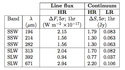
The plot below graphs the FTS point-source line flux sensitivity (unapodized; HR mode) as a function of wave number. The solid curve shows the most recent sensitivity measurement (June 2011), while the dashed curve is the previous one used in the first open-time proposall call (July 2010).
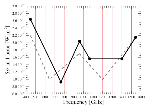
Remark: It has been tested that the noise level continues to integrate down as expected for about 100 scan repeats (100 forward and 100 reverse scans; total on-target integration time of about 3.7 hours). Beyond 100–120 scans, it is not observationally tested yet if the noise will go down as predicted.
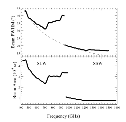
The effective beam profile of the spectrometer depends on the observed wavelength. While for the photometer the feedhorns could be designed to only accept one mode, the spectral range of the FTS has to allow for more modes entering the spectrometer feedhorn as the wavelength becomes shorter. This leads not only to an interesting structure of the transmission curve, but also to unusual variations in the beam profile over wavelength.
The FTS beam profile has been measured directly as a function of frequency by mapping a point-like source (Neptune) at median spectral resolution (see Makiwa et al. 2013, Beam profile for the HerschelSPIRE Fourier transform spectrometer, Applied Optics 52, 3864). The beam profiles of the SSW detectors are well represented by a radially symmetrical Gaussian function. In contrast, the beam profiles of the SLW detectors are not Gaussian. The resulting FWHM and associated solid angle of the beam as a function of frequency are shown in the plot below.
After having corrected for bolometer nonlinear responsivity, the bolometer voltage is in principle linearly proportional to the incident flux on the bolometer detector. This linearly bolometer voltage is Fourier transformed into the spectrum domain, with the resulting spectrum divided by a relative spectral response function (RSRF) to derive a flux-calibrated spectrum.
The basic flux calibration uses an RSRF based on the telescope model emission, which is a perfect extended source for the SPIRE FTS. The flux-calibrated spectrum has 3 contributors: (1) the astronomical target, (2) the telescope background, and (3) some instrument emission. Both (2) and (3) are then removed using modeled emissions.
For every sparse mode observation, a spectrum of point source flux calibration is also provided for the central detectors (SSWD4/SLWC3). The conversion from the extended-source flux calibrated spectrum to the point-source flux calibrated spectrum is based on a conversion factor determined from observations of Uranus and the wavelength-dependent beam sizes.
The primary flux calibration is dependent on a model of Uranus that has been compared to observations and models of Neptune and we find that overall the agreement between the models is better than 6% at all frequencies. This systematic error represents the overall absolute calibration accuracy of all FTS spectra. This is achievable for relatively bright point sources (> 100 Jy), assuming good telescope pointing and accurate background subtraction.
For fainter sources, other uncertainties might become relatively significant. These include errors from (1) imperfect telescope background removal, which is the dominant systematic error in point-source continuum (estimated to be on order of 0.3–0.5 Jy as HIPE 11), (2) imperfect instrument emission removal that affects only the long wavelength end of the SLW spectral segment, (3) flux error from the actual pointing offset resulting from the uncertainty in the target coordinates, and (4) contribution from the astronomical foreground or background at your target position. Note that only (3) may affect line flux errors, while all these factors affect the continuum flux accuracy.