You can choose from any of a wide variety of catalogs for overlaying on your visualized data.
Contents of page/chapter:
+Overview
+Catalogs from IRSA -- Overlaying catalogs
from IRSA
+Catalogs from disk -- Overlaying your own
catalogs
+Catalogs from VO -- Overlaying
catalogs obtained via the VO
+Columns and Filters -- Interacting with catalogs
+Plotting catalogs
Catalogs -- Overview
Once you have conducted a search and have some displayed images, you
can perform a catalog search, which will (among other things) overplot
those catalog sources on all the images shown. Catalogs are available
via a blue tab that appears at the top of the page only after you have
performed at least one search -- in essence, you need to have
something on which to overlay the catalog before it will let you
search.
Depending on how, exactly, you searched the NPA, you may already have catalogs returned by your search and overlaid on your images.
By default, it assumes you want to perform a catalog search that covers the same region as your currently selected target, and attempts to pre-fill the form with that region -- but you can choose to change those search criteria. You can choose from any of a number of catalogs, including but not limited to Planck catalogs. You can also upload your own catalogs.
The catalog will be overlaid on the images in the coverage pane as well as all of the channels shown in the image display pane. The highlighted source will change depending on which source is selected in the catalog tab in the results pane. When overlaying the sources from a catalog search, note that all the sources are shown.
By default, the catalog search page appears with a cone search approximating your prior search. You can customize the search for options beyond a polygon search (e.g., a cone search) by selecting from the "Search Method" drop-down. The entry box immediately to the right of that "Search Method" drop-down changes accordingly, and you can edit the parameters directly. If you choose a 'cone' search, you can also change the target by clicking on "Modify Target" next to the target center that appears. Caution: pick your units from the drop-down first, and then enter a number; if you enter a number and then select from the drop-down, it will convert your number from the old units to the new units. There are both upper and lower limits to your search radius; it will tell you if you request something too big or too small. Note that these limits are catalog-dependent.
You then need to specify the catalog you want to search. In order to
help it give you a specific list of choices, you need to first tell it
the project and category. After you have selected these items, on the
right, you can pick the specific catalog . To change catalogs, first
select the "project" under which they are housed at IRSA, such as
2MASS, IRAS, WISE, MSX, etc. The options under the "category" and the
specific clickable catalog on the right change according to the
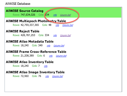
project you have selected. A short description is provided for each
of the catalogs, with links for more information (including
definitions of the sometimes cryptic column names); an example of this
link for more information is here:
You can also set restrictions on specific columns by clicking on "Set Column Restrictions" on the left hand side, under the "category" selection drop-down menu. A new window will open up with the available column names in the corresponding catalog, and you can choose what to display, and filter what is returned (for example, only return objects with values in column y that are greater than x). If you add more than one restriction, they are combined logically using an "AND" operators; be careful, because you can thus restrict data such that none of the catalog meets your criteria.
Power user tip: By default, this interface may show you fewer columns than are available in the full catalog. By clicking on "Set Column Restrictions" and selecting "long form" from the drop-down at the top of the pop-up window ("Please select long or short form display"), you can access the full range of available columns. In some cases, there are literally hundreds of columns that you can access!
Click on "Search" to initiate the search. It will load the catalog
into a tab of its own. The catalog objects will also be overlaid on
the images you have loaded. You can obtain a full-screen view of your
catalog -- click on the expand icon in the upper right of the window
pane when your mouse is in the window:  . You can also make an x-y plot from the
catalog (for more on the x-y plots, see below).
The images and the catalog representations are interlinked -- clicking
on a row in the table shows it on the images and vice versa.
. You can also make an x-y plot from the
catalog (for more on the x-y plots, see below).
The images and the catalog representations are interlinked -- clicking
on a row in the table shows it on the images and vice versa.
To close the catalog search window without searching on a catalog, click on "Close" in the upper left.
NOTE THAT the search may take a long time to return, especially if you have asked for a large catalog, and you may think that nothing has happened, but be patient and eventually it will either spin off to the background monitor (from which you can load it into a tab), or return a tab directly.
Searches that take longer than a few seconds get spun off to the background monitor. If it does spin off to the background monitor, it will dynamically update to reflect its status, and will let you know when the catalog is ready to download or display. A popup appears asking if you want to load the catalog. Either click on the popup or explicitly open the background monitor and click on the catalog name to load it into a tab of its own.
Use large search radii with caution! Be sure you understand how many sources you are likely to retrieve. Searches that retrieve more rows will take longer. Searches that retrieve millions of rows will take quite a while.
By clicking on the blue "Catalogs" tab, you are by default dropped into the interface for searching for catalogs at IRSA. However, you can pick another tab from the top left of the catalogs screen, "Load Catalog", to load your own catalog.
Your catalog needs to be in IPAC table format ![]() , which is a varietal of plain
text. IRSA has a table validator
, which is a varietal of plain
text. IRSA has a table validator ![]() which
may be helpful, or you can download just about any catalog you find
through IRSA, and copy that format.
which
may be helpful, or you can download just about any catalog you find
through IRSA, and copy that format.
Your table file MUST have RA and Dec values, and unless it is specified, it assumes J2000.
You can add a "SYMBOL" parameter to change the shape (X, SQUARE, CROSS, EMP_CROSS, DIAMOND, DOT) of catalog marks, e.g.:
\SYMBOL = X
You can add a "DEFAULT_COLOR" parameter to assign a CSS color name or a HEX value to catalog marks, e.g., either of these two:
\DEFAULT_COLOR = lightcyan
\DEFAULT_COLOR = #00FF00
You can find the CSS color code or the CSS color HEX values
Your catalog is then shown (and interacted with) in the same way as the other catalogs described here.
By clicking on the blue "Catalogs" tab, you are by default dropped into the interface for searching for catalogs at IRSA. However, you can pick another tab from the top left, "VO Catalog", to search for and load catalogs from the VO.
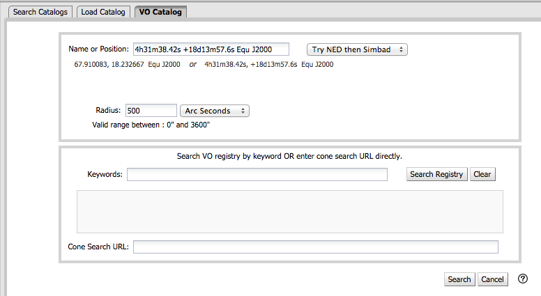
As for the IRSA catalog search, the tool pre-fills the target position with the coordinates of the target with which you have been working. In this case, you are limited to a cone search, so the next option is the cone search radius. As usual, pick your units from the drop-down first, and then enter a number; if you enter a number and then select from the drop-down, it will convert your number from the old units to the new units. There are both upper and lower limits to your search radius; it will tell you if you request something too big or too small.
If you know your VO URL already, you can jump down to the Cone Search URL box and type or paste your URL into the box and hit search.
More commonly, however, users do not know a priori which URL to use. Type your desired keywords into the keywords box and click on "Search Registry". All of the URLs it finds for your keywords within the VO registry service are shown in the box. Locate the one you want to use, and click on "Use" on the far left of the corresponding row. The "Cone Search URL" is populated properly for that catalog. Click on "Search" to initiate the search.
The search results are then shown (and interacted with) in the same way as the other catalogs described here.
Example
Load the tool. Search on IC1396. Go to the catalogs tab. Choose "VO
Catalog." It wants the root URL for a cone search. I click on "Find
Astronomical Data Resources", which takes me here ![]() .
Search on IPHAS. Get this page
.
Search on IPHAS. Get this page ![]() . Look for the complete catalog release
(not just one associated with one specific study). The name of the
catalog goes here
. Look for the complete catalog release
(not just one associated with one specific study). The name of the
catalog goes here ![]() . Hit the [+] to expand it. There is one URL
listed there, under "available endpoints for the standard interface."
Copy that URL and paste it into the search form. The IRSA tool will
append your coordinates and radius and return you a table.
. Hit the [+] to expand it. There is one URL
listed there, under "available endpoints for the standard interface."
Copy that URL and paste it into the search form. The IRSA tool will
append your coordinates and radius and return you a table.
Tips and Troubleshooting
Note that searching the VO means that you are using resources not specifically housed at IRSA, so servers may be down, or timeouts set, or limits on numbers of returned sources, etc., that are beyond our control. In most cases the solution is to specify as precise a search as possible. Here are the links to VO registries that we are using, just in case you want to do more flexible searches of the registry. The URL you enter into the box in FinderChart, though, must be a Cone Search base URL (not containing RA and Dec parameters, which are inserted into the URL by FinderChart in response to the search parameters you give it).
The master list of registries is here ![]() . You can also search the registries directly
via that link (as opposed to via the IRSA tools).
. You can also search the registries directly
via that link (as opposed to via the IRSA tools).
Columns and
filters -- Interacting with catalogs
After you have loaded a catalog, it appears as an additional tab in
the left-hand-side search results pane. Additional catalogs you load
appear as additional tabs in this window pane. To see more of the
columns, grab the divider between the two window panes and slide it
right to widen the pane.
The table is shown exactly as it appears in the corresponding database
(or as it appeared on your disk), with all columns as defined for that
catalog. To understand what each column is, please see the
documentation associated with that catalog. (For IRSA catalogs, this
documentation is available via the catalog searching popup window, see
figure below, or by navigating through the IRSA website.)
The tab (and table) name itself is the name of the catalog file as stored on the system at IRSA; it is a little cryptic, but the first few words should make it clear whether it is WISE, 2MASS, etc. To remove the tab, click on the blue "X".
Immediately below the tab name, there are several icons, just like in in the main search results. See table navigation in the Results section for details on what these icons do. You can also interactively impose filters from plots you make from the catalog - see the next section.
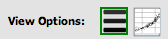 The first one is table view, and the second
is plot view. The current view is boxed in green. Click on the icon to
change views. If you do not see this icon, make sure that a catalog
tab is in the foreground of the target list pane. To see more of the
catalog while still viewing images, click and drag the slider between
the panes to enlarge the plot window pane.
The first one is table view, and the second
is plot view. The current view is boxed in green. Click on the icon to
change views. If you do not see this icon, make sure that a catalog
tab is in the foreground of the target list pane. To see more of the
catalog while still viewing images, click and drag the slider between
the panes to enlarge the plot window pane.
To obtain a full-screen view of your plot, click on the expand icon in
the upper right of the window pane when your mouse is in the window:
. To return to the prior view, click
the "Close" arrow in the upper left.
The plotting tool, by default, starts with RA and Dec plotted. Note
that it does so strictly mathematically correctly -- that is, RA
increases to the right (the reverse of astronomical convention). To
change what is plotted, click on the gears icon in the upper left of
the plot window:  . Configuration
options then appear to the left of the plot. You can choose a single
column to plot against another column -- if you have loaded a WISE
catalog, you could plot w1snr vs. w1mpro. You can start typing a
column name into the X and Y boxes, and it will help provide you
viable options from the column headings. Alternatively, you can click
on the "Cols" link to bring up a pop-up window with all the columns
for that catalog listed. NOTE THAT you must type in the column name
exactly matching the column headings as displayed. By
default, it echoes the x and y labels and units from the original
table, but you can change this by clicking on the triangles below each
entry box (e.g., make the label "SNR in WISE-1" rather than the more
cryptic column header "w1snr").
. Configuration
options then appear to the left of the plot. You can choose a single
column to plot against another column -- if you have loaded a WISE
catalog, you could plot w1snr vs. w1mpro. You can start typing a
column name into the X and Y boxes, and it will help provide you
viable options from the column headings. Alternatively, you can click
on the "Cols" link to bring up a pop-up window with all the columns
for that catalog listed. NOTE THAT you must type in the column name
exactly matching the column headings as displayed. By
default, it echoes the x and y labels and units from the original
table, but you can change this by clicking on the triangles below each
entry box (e.g., make the label "SNR in WISE-1" rather than the more
cryptic column header "w1snr").
You can also do simple mathematical manipulations. For example, if you
have loaded a WISE catalog, you can plot w1mpro vs. w1mpro-w4mpro.
However, note that as of this version, the axes are from min to max in
the strict mathematical definition of the term, so in this example,
the fainter W1 objects are at the top of the plot. As a workaround for
this, plot -w1mpro vs. w1mpro-w4mpro to get the axes aligned in the
way you are expecting such that brighter objects are at the top of the
plot.
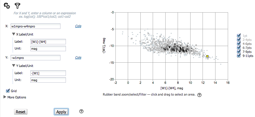
Note that the plot symbols are shades of grey corresponding to how many points are represented at that location in the plot. The lightest shade of grey (and smallest points) represent one point in the plot at that location, and the darkest shades of grey (and the largest points) represent many more points in the plot at that location. Put your mouse over any of the points to find out more about what is represented at that location.
You can add or remove the gridlines via the "Grid" checkbox. If you have zoomed in enough such that there are just black boxes -- one object per point -- you can change the plot style such that the points are connected or unconnected.
You can also restrict what data are plotted in any of
several different ways. You can set limits based on the "more options"
(click on the triangle next to "more options") on the lower left of
the plotting window pane, or you can use a rubber band zoom, as
follows. Click and drag in a sub-region of the plot. The icons in the
upper right of the plot change corresponding to what you can do, in
this case to these:  . They are, from
left to right: zoom in on the region you have selected, select the
objects in the catalog, filter the catalog to leave only those
objects, or expand the plot to take up the whole browser screen. If
you click on the zoom icon, then the plot axes change to encompass
just the sources you have selected. If you click on the select icon,
then the plot symbols corresponding to your selection change shape and
color, the corresponding objects overplotted on the image in the image
window pane change color, and (if you change back to the table view of
the catalog), the rows (corresponding to those sources) in the catalog
are highlighted. If you click on the filter icon, then the catalog
view is filtered down, restricted to just those sources you have
selected, and the filter notes in the upper left of the plot window
(and in the table view of the catalog) change to remind you that you
have a filter applied. Only those sources that pass the filter are
shown overlaid on the image(s). (This is the behavior of 'filter', as
opposed to 'select'; the former restricts what is shown, the latter
just highlights the objects.) For more on filters, see the filter section.
. They are, from
left to right: zoom in on the region you have selected, select the
objects in the catalog, filter the catalog to leave only those
objects, or expand the plot to take up the whole browser screen. If
you click on the zoom icon, then the plot axes change to encompass
just the sources you have selected. If you click on the select icon,
then the plot symbols corresponding to your selection change shape and
color, the corresponding objects overplotted on the image in the image
window pane change color, and (if you change back to the table view of
the catalog), the rows (corresponding to those sources) in the catalog
are highlighted. If you click on the filter icon, then the catalog
view is filtered down, restricted to just those sources you have
selected, and the filter notes in the upper left of the plot window
(and in the table view of the catalog) change to remind you that you
have a filter applied. Only those sources that pass the filter are
shown overlaid on the image(s). (This is the behavior of 'filter', as
opposed to 'select'; the former restricts what is shown, the latter
just highlights the objects.) For more on filters, see the filter section.
If you move your mouse over any of the points, you will get a pop-up telling you the values corresponding to the point under your cursor. If you click on any of the points, the object(s) corresponding to that point will be highlighted in the overlays in the images shown, and highlighted in the catalog table view of the catalog. This works the other way too - click on a row in the catalog, or an object in the images, and the object will be highlighted in the plot or the catalog or the image.
If you have a very large catalog or many points in a particular location of the plot, the tool will rebin the points in the plot such that displaying the plot is faster. The plot symbols are shades of grey corresponding to how many points are represented at that location in the plot. Put your mouse over any of the points to find out more about what is represented at that location. It will tell you how many catalog rows correspond to that point, and clicking on it will highlight all of the corresponding rows in the table view and the image overlays. In order to have the tool plot one point per row, you need to zoom in or otherwise restrict the data such that there are 'few enough' points represented in the plot. If there is just one point in the plot that needs to be rebinned, all of the points will be a small point.
Want to save a plot to file? At this time, the best way to do that is a screen snapshot. On a Mac, this is accomplished via holding down command, then shift, then 4, then let go and your mouse cursor changes. Hit the space bar to select the window over which your mouse is hovering. Your mouse cursor changes again, and hit the mouse button. A snapshot is then saved to your Desktop, tagged with the date and time.
Once you have made an x-y plot, the plot is then effectively treated as another 'image' in the stack of images you have loaded into the tool. In the Visualization section, it describes various features, including blinking images, and removing images from the blink sequence. If, after you make a plot, you want to blink or tile some of the FITS images, you will need to remove the plot from the image sequence, as described in the Visualization section.