SPHEREx Data Explorer: Spectrophotometry Tool
Every location in a SPHEREx image has a unique ra, dec, and
wavelength. Doing photometry on SPHEREx images therefore is actually
spectrophotometry. This spectrophotometry tool is integrated into the
SPHEREx Data Explorer, building on core capabilities of Tables, Plots, and Spectra. Generic help on those capabilities
can be found in those other sections; this section is specific to the
Spectrophotometry Tool. The first few subsections explain how the
tool works conceptually, while the later subsections provide
step-by-step instructions for running it.
Contents of page/chapter:
+Introduction
+Background
+Fitting Modes
+Data Inputs
+Implementation Overview
+Outputs
+Initiating a Process <-- Jump here
to learn more about starting a job
+Job Monitor
+Results
+Exploring Bitflags
+Saving Results
+After SPHEREx
+Different Behaviors: Loading from the
Job Monitor, Pinning, and Loading from Disk
+Tips for Success
The SPHEREx Spectrophotometry Tool measures fluxes across multiple
SPHEREx Spectral Images to generate a low-resolution near-infrared
spectrum for any specified sky position. You need to provide the
known positions of sources. The Tractor
 performs forced photometry
by modeling how sources would appear in SPHEREx images using the
measured PSF, and calculates the best estimate of their fluxes.
performs forced photometry
by modeling how sources would appear in SPHEREx images using the
measured PSF, and calculates the best estimate of their fluxes.
The tool supports two models for the intrinsic source morphology
(i.e., the source structure before convolution with instrumental
effects or the SPHEREx PSF):
- Point Source
- Sérsic Galaxy Profile
Processing takes longer when more SPHEREx spectral images include the
positions you want to analyze. Spectrophotometry for a single source
(comprising individual forced photometry measurements from all SPHEREx
images containing the source) can take anywhere from minutes to hours.
Sources near the ecliptic poles, which have the deepest coverage, can
have of order ~2e4 individual measurements and may require several
hours of processing. The tool is currently limited to a relatively
small number of sources per run.
If a source of interest is known to have a close companion, they can
be fit simultaneously with Tractor by providing the coordinates of
both sources. This approach can mitigate the impact of blending on the
recovered flux of the source of interest.
The SPHEREx Spectrophotometry Tool uses The Tractor
to perform forced
photometry on sources at specified positions. It combines
user-provided source positions and intrinsic morphologies with
instrument characteristics (point-spread function, pixel response, and
noise) to produce robust, deblended SPHEREx spectrophotometry. Tractor
predicts the observed image from these inputs and adjusts the free
parameters (the source fluxes) to best match the data. Although
Tractor can fit a background level, the Spectrophotometry Tool applies
a separate background-subtraction step before photometry.
The SPHEREx Spectrophotometry Tool considers two models for the
intrinsic source. In both cases, only the source flux amplitude is
fitted by the tool; all other source parameters must be provided by
the user and remain fixed.
- Point Source
- The intrinsic source is treated as a delta function located at the
user-specified position.
- Sérsic Galaxy Profile (or Sérsic Profile )
- The intrinsic source is modeled as an extended galaxy. Users must
provide the following fixed parameters:
- Sérsic index (n): 0.5 ≤ n ≤ 6. While some galaxies may be
well-characterized by more extreme values, the allowed range includes
the values over which the tool has been tested.
- Minor-to-major axis ratio (b/a): 0 < b/a ≤ 1.
- Position angle (PA): -360 degrees ≤ PA ≤ 360 degrees, measured
east of north.
- Effective radius (Re): 1 ≤ Re < 20 arcsec. Values below 1
arcsec are interpreted as a point source.
In addition to the parameters provided by the
user, the SPHEREx Spectrophotometry Tool requires several data
products for each source. These are automatically retrieved by the
tool, so the user does not need to provide them manually.
The primary data come from the SPHEREx Quick Release Spectral Images
(version 2), which are multi-extension FITS files with the following
extensions:
- IMAGE: Per-pixel flux in MJy/sr.
- FLAGS: Pixel-level flags indicating issues such as saturation or
strong non-linearity, as well as pixels containing flux from known
sources so they can be masked when estimating the local background.
- VARIANCE: Per-pixel uncertainty estimates corresponding to the
spectral image.
- PSF: The high-resolution, position-dependent point spread function
for the corresponding detector region.
- ZODI: (Not used by the tool.)
In addition, the tool uses the Pixel Solid Angle Map, derived from the
distortion map, to convert fluxes to μJy.
These inputs, together with the user-specified intrinsic morphology
parameters, allow the tool to accurately fit source fluxes and
propagate relevant flags to the output catalog.
The SPHEREx Spectrophotometry Tool performs forced photometry on
sources with known positions and user-provided intrinsic morphology
parameters. Only the source flux amplitude is fitted; all other
parameters are held fixed. The tool automatically retrieves the
required SPHEREx data products, so users do not need to manage them
manually.
For each source, the tool:
- Extracts a cutout from the IMAGE extension of the SPHEREx Quick
Release Spectral Image, centered on the source (per-pixel flux in
MJy/sr).
- Computes and removes a local background from nearby pixels,
masking pixels flagged in the FLAGS extension as containing flux from
known sources.
- Retrieves the position-dependent PSF from the PSF extension for
the cutout region.
- Uses Tractor to fit a generative model combining the source's
intrinsic morphology and the local PSF, adjusting only the source flux
amplitude. The fit uses per-pixel uncertainties from the VARIANCE
extension.
- Converts fitted fluxes to μJy using the Pixel Solid Angle map.
- Propagates pixel-level flags from the FLAGS extension to the output
catalog and applies additional photometry-specific flags for issues
such as strong non-linearity or saturation.
- Computes a fit quality metric based on the residuals between the model
and the spectral image within a 2.5-pixel radius aperture; values near
1 indicate good fits.
The Spectrophotometry Tool produces a table, which includes the
spectrum.
- Core Spectral Columns
- These provide the fundamental science spectrum.
- wavelength (μm) -- Wavelength at which photometry was measured.
- flux (μJy) -- Source flux density.
- flux_err (μJy) -- Uncertainty on the flux measurement.
- lambda_width (μm)-- Effective bandpass width associated with the wavelength measurement.
- Quality Assessment Columns
- These help you evaluate the reliability of each flux measurement.
- flags -- This column contains an integer bitmask value
representing issues that affected the photometry measurement. Each bit
in the value corresponds to a specific condition, and multiple
conditions are represented as the sum of their corresponding bit
values. To determine which conditions apply, convert the flag value in
the output to binary and examine the bits that are set. Detailed
definitions of each bit are provided below and in the Explanatory
Supplement, available from the SPHEREx Mission Page.
- fit_ql -- Photometry quality metric. For each source, a circular
region of radius 2.5 SPHEREx pixels around its subpixel position is
used to compute:
fit_quality = < |p_k - m_k| / sigma_k >
where p_k is the pixel value in the Level 3 image, m_k is the Tractor
model value, and sigma_k is the per-pixel uncertainty from the
variance map. Values near 1 indicate good fits; larger values suggest
potential problems.
- flux_bkg -- Background flux estimate used in the fit.
- Provenance Columns
-
These identify the exposures and detectors that contributed to each spectral point.
- lvf_id -- ID of the LVF exposure used for photometry.
- det_id -- Detector ID.
- deep_flg -- True if the measurement is from a Deep Field.
- mjd -- Modified Julian Date of the exposure.
- Inspection Columns
- These columns indicate where the requested position falls in each overlapping spectral image.
- x_image, y_image -- Pixel coordinates of the requested position
within the spectral image used for the photometry measurement, derived
from the image WCS.
- ra, dec -- Sky coordinates corresponding to the same position.
Bit-level flags are set in the images and are propagated through the
spectrophotometric process to indicate if the spectrophotometric
measurement may be affected by any pixel-level flags. If any pixel in
the constituent images is flagged, then that flag is carried over into
the resultant spectrophotometric measurement flag. The number of
impacted pixels is currently not returned.
| Name | terse definition(*) | Python expression | value expression |
value | can appear in images? | can appear in spectrophot
output? |
|---|
| TRANSIENT | e.g., CR hit | 1 << 0 | 2^0 | 1 | yes | yes |
| OVERFLOW | nearing saturation | 1 << 1 | 2^1 | 2 | yes | yes |
| SUR_ERROR | possible errors | 1 << 2 | 2^2 | 4 | yes | yes |
| PHANTOM | | 1 << 4 | 2^4 | 16 | yes | yes |
| REFERENCE | | 1 << 5 | 2^5 | 32 | yes | yes |
| NONFUNC | dead pixel | 1 << 6 | 2^6 | 64 | yes | yes |
| DICHROIC | unusable pixel | 1 << 7 | 2^7 | 128 | yes | yes |
| MISSING_DATA | no data | 1 << 9 | 2^9 | 512 | yes | yes |
| HOT | noisy pixel | 1 << 10 | 2^10 | 1024 | yes | yes |
| COLD | dead pixel | 1 << 11 | 2^11 | 2048 | yes | yes |
| FULLSAMPLE | full history avail | 1 << 12 | 2^12 | 4096 | yes | yes |
| SUR_MISMATCH | | 1 << 13 | 2^13 | 8192 | yes | yes |
| PHANMISS | can't be corrected | 1 << 14 | 2^14 | 16384 | yes | yes |
| NONLINEAR | can't be corrected | 1 << 15 | 2^15 | 32768 | yes | yes |
| VAR_UNDER | | 1 << 16 | 2^16 | 65536 | yes | yes |
| PERSIST | persistent charge | 1 << 17 | 2^17 | 131072 | yes | yes |
| PERSIST_UNK | | 1 << 18 | 2^18 | 262144 | yes | yes |
| OUTLIER | flagged outlier | 1 << 19 | 2^19 | 524288 | yes | yes |
| CROSSTALK | | 1 << 20 | 2^20 | 1048576 | yes | yes |
| SOURCE | known source | 1 << 21 | 2^21 | 2097152 | yes | yes |
| GHOST | | 1 << 22 | 2^22 | 4194304 | yes | not yet |
| GHOST_EXT | | 1 << 24 | 2^24 | 16777216 | yes | not yet |
| BLOOM | | 1 << 26 | 2^26 | 67108864 | yes | not yet |
| SNOWBALL | | 1 << 27 | 2^27 | 134217728 | yes | not yet |
| HALO | | 1 << 28 | 2^28 | 268435456 | yes | not yet |
| SATELLITE_HALO | | 1 << 29 | 2^29 | 536870912 | yes | not yet |
| CONTAINS_BAD_PIXEL | bad pixel involved | 1 << 32 | 2^29 | 4294967296 | no | yes |
| FIT_ERROR | error in fitting | 1 << 33 | 2^33 | 8589934592 | no | yes |
(*) for full definition and discussion, see the Explanatory Supplement on the SPHEREx Mission Page
See Exploring Bitflags below for how to
explore bitflags using this tool.
Some bits are not listed here; those bits are used in products not
publicly released.
The tool keeps track of whether the photometry included any "bad" pixels
(defined by the list above) using the CONTAINS_BAD_PIXEL (bit 32)
flag. This provides a convenient way of selecting down to only
measurements unaffected by known problematic effects. In other words,
if the bitflag is a very large number, 4294967296 or more, then that
point is problematic.
The existence of any of these flags in the measurement should be
considered a warning when using / interpreting the point, and do not
necessarily mean that the measurement is unusable. However, there are
two exceptions. The first is DICHROIC (bit 7). Currently the
calibration in the dichroic region is not perfect, and users would be
advised to be skeptical of these measurements until further refinement
of the absolute calibration. The second exception is FIT_ERROR (bit
33), indicating a failure to converge.
Pixels with any of the following flags will be ignored when fitting
with Tractor:
- SUR_ERROR
- NONFUNC
- MISSING_DATA
- HOT
- COLD
- NONLINEAR
- PERSIST
Note on background: The
background estimated under the source is returned with the photometry
as "flux_bkg". The background can be problematic in some (rare) cases,
and the methodology will be improved in the next version of the
pipeline. Users are advised to check for sharp discontinuities between
adjacent wavelengths in the background estimates if they suspect an
issue with their photometry result.
The screen from which you initiate a spectrophotometry process looks
very much like the Spectral Image Search
but it is different.
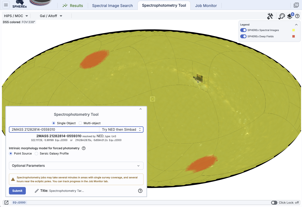
Just like in a Spectral Image
Search, you have a HiPS
image loaded that takes up most of the browser area. Overlaid on
top of the HiPS image, there is a MOC indicating the sky coverage for
the data currently available in the archive, and one for the deep
fields coverage. As you zoom in, the shaded regions become more
transparent, or you can change them in the layers pop-up.
Again, just like in a Spectral Image Search, you can enter a single target or upload a list of targets; please see
that section for details of how to do that.
And, just like in a Spectral Image Search, these spectrophotometry
jobs are managed in the Job
Monitor. If you are submitting a lot of jobs, keeping track of
which job is which in list in the Job Monitor can be difficult. Using
the "Title" field near the bottom of the spectrophotometry window, you
can change the title by which the search will be listed in the Job
Monitor. You don't have to change it from the default to be able to
submit jobs, however. (Once you change it, though, all subsequent
jobs you make will still have that same title unless you change it
each time.)
Point Sources

|
As discussed above, one of the two modes the tool supports is point
sources. You specify the necessary parameters here. At minimum, you
just provide the location(s), and let it take the rest of the default
parameter values; the defaults work fairly well.
⚠ Tips and
Troubleshooting
- Parameters: The tool doesn't recenter the
position(s), so be sure you are providing a good location(s).
- Nearby sources:
- If there is a nearby, potentially confused source (recall
SPHEREx's pixels are ~6 arcsec; see the Explanatory Supplement on the SPHEREx Mission Page), you need to provide the tool the locations of all
of the sources you want to deconvolve. Upload a list of targets with
all of the sources included.
- However, if there are sources within the 15 px box that the tool
uses for background estimation, you do not need to
specify those; the tool knows about bright sources all over the sky.
(See the Explanatory Supplement on the SPHEREx Mission Page)
- Selecting all wavelengths or no wavelengths has the same effect --
it will attempt to provide all the data it can find. If you select
just one (or a few) range(s) of wavelengths, it will do only what you request.
- Run time:
- The more frames the tool has to work through, the longer the
process will take. If you ask for a source near the ecliptic poles,
where there might be at least one image per orbit, it will take a long
time for the tool to work through all the images to get a spectrum. If
you ask for a source near the ecliptic plane, where there are far fewer
images, the process will complete relatively quickly.
- If you submit a list of targets all over the sky, it will take a
long time for the process to run. If you submit a list of targets
close together on the sky, the tool is clever enough to only pull the
images it needs once, and obtains fluxes for all the sources at the
same time.
- A back-of-the-envelope calculation for run time is as follows --
do an image search to figure out how many images cover your target.
Then, to obtain the estimated run time in seconds, calculate
1.67*number images + 50; for run time in hours, calculate
0.000463*number images + 0.013.
- Throttles: To allow computing resources to be
shared fairly among all users, there are built-in throttles.
- You are currently allowed a maximum of two spectrophotometry jobs
running simultaneously. Additional jobs will be queued and run when
resources are available.
- Lists of targets are currently limited to 20 sources.
- Additional tips for success are below.
|
Sérsic Galaxy Profile

|
As discussed above, one of the two modes the tool supports is
Sérsic Galaxy Profile. You MUST specify all the necessary
parameters here.
You can submit a list of targets here too; if you upload a catalog,
there should be columns for all of the necessary Sérsic
parameters, and you will be asked to indicate which column from your
input catalog should be used for these values.
⚠ Tips and
Troubleshooting
- Parameters:
- The tool only fits the
flux; it takes from your input the position, the
Sérsic index, the major/minor axis ratio, position angle, and
effective radius. Be sure you are providing good values for these
parameters.
- Selecting all wavelengths or no wavelengths has the same effect --
it will attempt to provide all the data it can find. If you select
just one (or a few) range(s) of wavelengths, it will do only what you request.
- Run time:
- The more frames the tool has to work through, the longer the
process will take. If you ask for a source near the ecliptic poles,
where there might be at least one image per orbit, it will take a long
time for the tool to work through all the images to get a spectrum. If
you ask for a source near the ecliptic plane, where there are fewer
frames, the process will complete relatively quickly.
- If you submit a list of targets all over the sky, it will take a
long time for the process to run. If you submit a list of targets
close together on the sky, the tool is clever enough to only pull the
images it needs once, and obtains fluxes for all the sources at the
same time.
- Throttles: To allow computing resources to be
shared fairly among all users, there are built-in throttles.
- You are currently allowed a maximum of two spectrophotometry jobs
running simultaneously. Additional jobs will be queued and run when
resources are available.
- Lists of targets are currently limited to 20 sources.
- Additional tips for success are below.
|
Multiple targets
Once you select "Multi-object", if you haven't yet uploaded a table,
you get the upload pop-up window, from which
you can upload a file. That upload section
contains more information about file formats, etc.
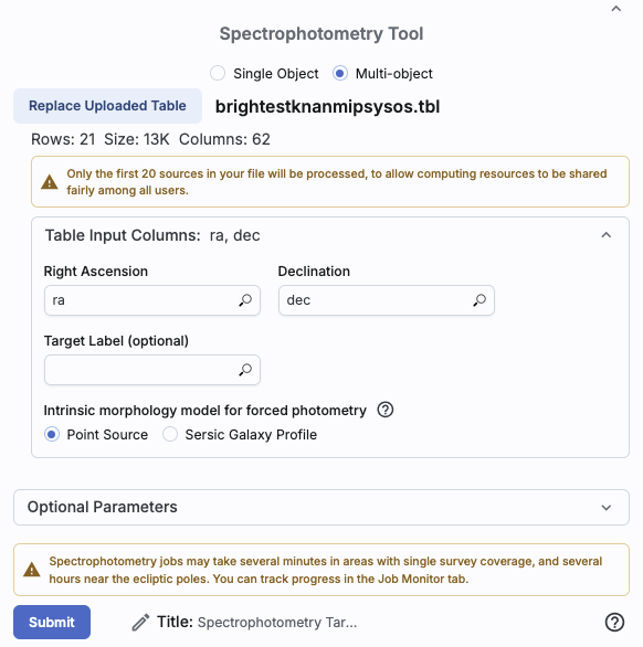
|
If you have columns "ra" and "dec", the upload tool may be able to
guess that those are the position columns. If it can't guess the
position columns, or it guesses incorrectly, then you can select from
the uploaded columns by selecting the magnifying glass and choosing
the correct column from the available columns it provides. You can
also choose to select a target label from your uploaded table; this is
optional.
The "optional parameters" for multiple targets are the same as for
single targets, and apply equally to all of the uploaded targets.
⚠ Tips and
Troubleshooting
- If your list has more than 20 sources, as the one in the
screenshot here does, then the tool will only take the first 20
sources. Break your list into sets of 20 to submit them.
- If you are submitting a list for Sérsic Galaxy Profile
fits, you should provide additional columns for the Sérsic
parameters; just like for the ra and dec columns, you can teach the
tool which columns to use for these parameters.
- Related to the prior item: You can't upload a list of targets and
pick the same Sérsic parameters from the target submission
screen for all the targets at once. Your uploaded catalog has to have
values for each of the Sérsic parameters.
|
Any spectrophotometric job, even a point source with minimal
wavelength coverage, takes measurable time (at least 5 minutes).
Therefore, you should send the job to the Job Monitor.

Click on "Send to Background", and the job monitor will take over
management of the job; you can then continue to work in the tool while
you wait. See the Job Monitor section
of the Downloads chapter for more information.
After a spectrophotometry job finishes in the Job Monitor, click on
the icon that matches that in the "Results" tab  to display the results of this job in the
tool.
to display the results of this job in the
tool.
Here are the results of a spectrophotometry run on a single
target:

On the left is a list of all the requested targets (here, only one),
and on the right, the "Data" tab is in the foreground with the
extracted spectrum plotted. Across the bottom of the screen are
cutouts from the constituent images, centered on the target.
The plotted spectrum has some properties like that of generic plots in this tool, but because the tool
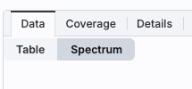
realizes that it is a spectrum, it has some properties that are specific to spectra. Moreover, if you click on
the table/spectrum toggle in the upper left of the right hand pane,
you can view the spectrum as a table. Then you can interact with the
spectrum as you can with any other table in this
tool.

All the columns that the tool produces are defined above.
The images at the bottom and the plot (or table) are linked. If you
click on a point in the plot, the cutouts are updated to reflect your
selection. In general, the currently selected point is the center
cutout in the display. From the row immediately above the images, you
can set the number of images shown at the same time via radio buttons
( ), set the size of the cutouts (
 ) where the default is 1.2 arcmin, and
control whether or not the cutouts are linked together by WCS (
) where the default is 1.2 arcmin, and
control whether or not the cutouts are linked together by WCS ( ) where they are linked together by default.
The image toolbar works here just as for all other images in this tool.
) where they are linked together by default.
The image toolbar works here just as for all other images in this tool.
This is what the results look like for a submitted list of targets --
very similar to that for a single target, but with multiple targets on
the left.

The flags that are returned by the spectrophotometry calculation are
important. You can use this tool to explore what flags are set, and
why, in several different ways.
Look at the flags column
This is the simplest and easiest thing to do. As described above, you
can view the spectrum as a plot or a table. Change your view of the
spectrum to a table, and look at the values in the "flags" column. To
first order, big is bad. 0 is good. In more detail, measurements with
flag values of 0 (no flags) or 2097152 (source mask) include only
pixels in a nominal state. Bit 29 (4294967296) means something in the
spectrophotometry calculation from that image involved a bad pixel. So
anything that starts with 429xxxxxxx is something to be suspicious
about. You can sort the table by the flags to be in descending order,
or filter out the largest numbers. This screenshot has the flags
column sorted in descending order. (29 of the 176 points in this
particular spectrum have that bit set.) The 'source' bit, bit 21
(2097152) could be nominal, but depending on context, could suggest
that source contamination could be important. You can then decide on a
case-by-case basis what to investigate in more detail.

You can also change the color of the points in the spectrum plot to
correspond to the flags column -- this
example shows how to change the plot point colors to correspond to
the dates of the observation, but you can do the same sort of thing to
make the colors correspond to the flags column. Then, as you move your
mouse over each point in the plot, the pop-up will tell you the value
of the correpsonding flags value. (The string "#this" is a
strange-looking IVOA term that means "the main data
product.")

Look for the dichroic flag
The dichroic flag only matters between bands 3 and 4. So, in order to
see any cases where this flag might be set, you need to filter down
the list of points in the spectrum that are from bands 3 or 4.
As described above, you can view the spectrum as a plot or a table.
Change your view of the spectrum to a table and look for the column
called "obs_publisher_did." This is the field that the tool uses to go
find the images it shows at the bottom of the screen -- it is
basically a link to the images. But the images have the band in the
filename! Turn on the filters if they're not on already, and add a
filter for the strings "D3" or "D4" in obs_publisher_did, e.g.,
like '%D3%' or like '%D4%'
Then, only the photometry points that emerged from bands 3 or 4 will
be left in your table, and you can then inspect the 'flags' value for
them individually using one of the other techniques here.
Look at the images
Because this tool automatically pulls the images for you, AND can
automatically overlay the masks, it becomes really easy to inspect
each constituent image.
As described above, the tool pulls the cutouts for each of the
constituent points in the spectrum and shows them to you along the
bottom of the window. As described in the Visualization chapter, you can
control the layers that are shown on your images. At the bottom of the
layers pop-up, you can enable the mask layer. Do it, and turn on all
of them ("show all") but then turn off bit 21 ("Source"). You'll be
left with color-coded indications of which pixels might be
problematic:

In this example, the selected row has flags = 4297064449, suggesting
that something might be questionable about this point. The
corresponding image is the one outlined in brown at the bottom.
Indeed, one of the points involved in the source appears to have been
affected by a something flagged as a transient -- the red pixel.
In this fashion, you can then decide on a case-by-case basis what to
investigate in more detail.
Decode the flags
Because you have the spectrum available as a table, you have all the table capabilities
available to you. This means you can create new columns in the table,
and you can manipulate the flags table to create new columns that
indicate which bits are included.
Change your view of the spectrum to a table. Following the add column instructions, add a new
column to the spectrum table. Call the new column something useful
like BITN, where "N" is the number of the bit you are exploring.
For the expression, enter:
MOD(FLOOR("flags" / POWER(2, N)), 2) = 1
where N is again the number of the bit you are exploring. So, for
OVERFLOW (BIT=1), use MOD(FLOOR("flags" / POWER(2, 1)), 2) = 1.
Make sure to cast the data type as a long integer. Then 'add
column'.
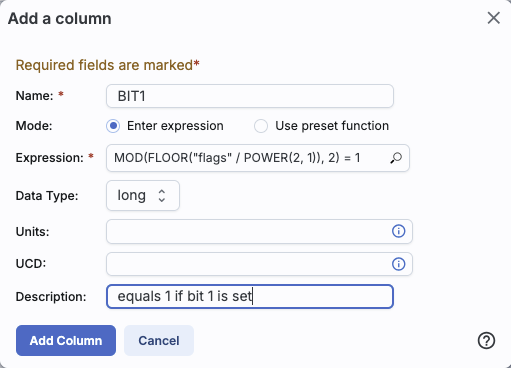
The new column will be 1 if that bit is set, and 0 if it is not. You
can create as many new columns as you need to explore which bits are
set.
Investigate background fluctuations
The note on background estimates above suggests
that you should investigate the background fluctuation. Use the plotting capability to change what is plotted,
though you have to work within the spectral
constraints. Go to the gears and ask it to plot flux_bkg rather
than flux. (The labels won't change, but you're doing explorations at
the moment anyway). If you get a plot with large changes, then it's
probably worth exploring in more detail. The linkages to images still
work, so the source in this screen shot has the substantial outlier
selected in the plot and highlighted in the cutouts along the bottom,
all set up for further exploration. (Because the labels don't change,
just be sure to set the plot back to 'flux' before you forget you've
changed it to flux_bkg!)

Export it and explore with Python
You can also download your spectra, load
it in to your suite of python code, and explore the data that way.
The existence of any of these flagged pixels in the photometry
measurement for a source can be tested using the "flags" field --
for example, to see if a source measurement included any
pixels flagged dichroic, do:
dichroic = 1 << 7
phot_flags = phot_result["flags"]
idx_dichroic = np.where(phot_flags & dichroic)[0]
There are several different ways to save the results from a
spectrophotometry run.
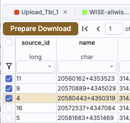
- Saving from the left pane
- (This is the method that is just like the Spectral Image Search
results as well as most like what you find in other IRSA tools with
this look and feel.) From the Results tab, in the left pane, just like
with the Spectral Image Search or other IRSA tools, select the rows
you want to download, and then select "Prepare Download." From there,
it's the same as other downloads
here. This is the best way to save the data.
Note that the filenames of the downloaded files are of the form
[ra]_[dec].xml but they are actually *.vot (VO tables), which is a
subcategory of XML files. (Note also that if you use the diskette to
save this table, you are only saving the table itself, not the data
that spring forth from this table, e.g., the spectra.)
- Saving the plot
- (This works just like saving any other
plot.) Click on the diskette icon in the upper right of the plot
pane to save the plot.
- Saving the table from the plot
- (This is somewhat more obscure than the above options, but works
just like saving any other table.) In
the top left of the plot, use the toggle that allows you to see the
spectrum as a table. Click on the diskette icon in the upper right of
this new table pane to save this spectrum table.
- Saving the results from the Job Monitor
- (This is much more obscure than the above options, but works in a
pinch if for some reason the results can't be loaded into the tool.)
Go to the Job Monitor tab, and
click on the info icon (
 ).
From that pop-up, click on 'Results' to expand that section, then
click on the link or click on the clipboard icon to copy the link and
paste it into a new browser. Then you can save the file that is loaded
into your browser (probably your browser's "File" menu then "Save
as"). If you save the file this way, it arrives in an xml vot format
(and you can't control that format; this is sort of an emergency
save).
).
From that pop-up, click on 'Results' to expand that section, then
click on the link or click on the clipboard icon to copy the link and
paste it into a new browser. Then you can save the file that is loaded
into your browser (probably your browser's "File" menu then "Save
as"). If you save the file this way, it arrives in an xml vot format
(and you can't control that format; this is sort of an emergency
save).

⚠ Tips and
Troubleshooting
- The Job Monitor is supposed to hold on to your jobs for 14 days,
but in testing we have found some transient gremlins suggesting that
(a) you should download the data as soon as you can; (b) logging in
before submitting your jobs (and before attempting to download the
results) seems to keep the gremlins at bay for longer.
- IRSA tends to have scheduled blocktimes every other Tuesday
morning Pacific time. Those blocktimes may take down our servers and
terminate running jobs and/or lose old jobs. We are working on ways to
ameliorate this, but, again, it's probably wise to download your data
as soon as possible.
- This spectrophotometry process takes a long time, with a lot of
disk i/o. Lots of people are accessing IRSA's servers in general, some
of whom in recent months have been malicious. We are working as fast
as we can to block the malicious and shift more resources to SPHEREx;
we thank you for your patience. You can also consider using SPHEREx data in the cloud . (There are Python Notebook tutorials .)
After you download the extracted spectral
data, you can upload the saved file into any of a number of tools,
including back into the SPHEREx Data Explorer (though see next
section).
Another tools that can read any of the files written by the SPHEREx
Data Explorer is IRSA Viewer
, which also has special
capabilities for handling spectra. Currently, some additional
capabilities are available in IRSA Viewer which are not present in
this SPHEREx tool. However, IRSA Viewer doesn't have all of the
SPHEREx-specific capabilities of this SPHEREx tool.
⚠ Tips and
Troubleshooting
- If you're in a situation where you've saved your spectrophotometry
results as an XML or VOT file, but you don't have any software ready
to read that, you can use IRSA Viewer to convert the XML or VOT file into
something else, like tbl or FITS format.
Once you start playing around with the Spectrophotometry Tool, you may
discover some apparent inconsistencies with how the tool is behaving.
There is method to the madness.
If you just let the tool run and don't explicitly put the
spectrophotometry job in the background, the results will be
automatically loaded into the tool, complete with cutout images.
If you put the spectrophotometry job in the background, once it
finishes, you'll have to click on the little green plot icon in the job
monitor to load the results into the tool, and the results will be
loaded into the tool, complete with cutout images.
If you come back to the same browser session on the same computer
anytime within the same few days, you can still click on the same
little green plot icon in the job monitor to load the results into the
tool, and the results will be automatically loaded into the tool,
complete with cutout images.
When you load the results this way, the linkage to the images
is preserved, and the tool understands how to get the
images.
Potential confusion #1.
If you have requested a set of <20 sources, then you will get the
list of sources on the left and the spectrum corresponding to each
object on the right. Or, if you have multiple single spectrophotometry
results loaded in different tabs on the left, as you change what you
have in the foreground on the left, the spectrum on the right
changes.
Each time you change what you've clicked on the left, it reloads
the entire data product on the right. So, if you impose a filter
on the plot or the data table, that filter is removed when you go back
and reload the data product. In order for the filter to "stick", you
need to first pin the spectrum ( ), and then filter the table associated
with that pinned spectrum. Then the filter persists even if you click
away from that spectrum and then come back to it. However, pinning
breaks the linkage to the images -- you no longer have the direct link
between the spectrum and the cutouts.
), and then filter the table associated
with that pinned spectrum. Then the filter persists even if you click
away from that spectrum and then come back to it. However, pinning
breaks the linkage to the images -- you no longer have the direct link
between the spectrum and the cutouts.
Potential confusion #2.
If you want to save the spectrum, in general, you need to use the
"prepare download" button, not the diskette icon. The diskette icon
usually saves just the table you're looking at. If you are looking at
the data table corresponding to the spectrum, you're fine using the
diskette, but if you're looking at a table that lists your source(s),
it will save that table and it won't save your spectrum/a.
Potential confusion #3.
If you download your spectrum, it's most likely going to save as an
XML file. If you turn right around and upload it back into this tool
via the upload tab, it will behave as if you
have pinned the spectrum -- that is, the linkage to the images is
lost. However, it will understand how to interpret the spectrum and
treat the errors, etc. properly.
For a spectrophotometry job loaded directly from the job monitor, the
"data" tab has the spectrum and "active chart" has a boring ra/dec
plot (with a single point). For spectrophotometry results loaded from
an xml file, "active chart" has the spectrum. "Data" may attempt to
grab one image, but will not know how to grab all of the images
corresponding to all of the images that went into the spectrum.
If you upload the XML file into IRSA Viewer (the more generic IRSA tool with this look and feel),
you have to warn it that the file contains a spectrum, and then
"active chart" plots the spectrum. It doesn't have any idea how to
retrieve the images, though it behaves as if it is trying to do so.
In this section, we have tried to collect all of the most important
tips for success in using this tool. We recommend reading, at the very
least, all of the information on this page about how the
spectrophotometry tool works, and ideally you should also consult the
Explanatory Supplement on the SPHEREx Mission Page.
- Parameters:
- The tool only fits the
flux; it takes all the other inputs from you.
- The tool doesn't recenter the
position(s), so be sure you are providing a good location(s). Did your
source move between its epoch and equinox (is it a high proper motion
source)?
- For galaxies, you need to provide not only the position, but also
the Sérsic index, the major/minor axis ratio, position angle,
and effective radius. Again, it doesn't fit those, so you need to
provide good values for these parameters.
- If you upload a catalog, there should be columns for all of the
necessary Sérsic parameters, and you will be asked to indicate
which column from your input catalog should be used for these
values.
- For single sources, there is error trapping when you input
parameters, but when you upload a list of targets, there isn't error
trapping. If you ask it to calculate fits where the Sérsic
parameters aren't physical, it will still attempt to do this.
- The drill is not a spectrophotometry run.
- The Mosaic Tool is the newest SPHEREx tool,
and it runs to completion much more quickly than the Spectrophotometry
Tool. It generates a FITS cube, where each plane is a different
wavelength. You can use the extraction tools to very quickly
drill through the cube to generate a spectrum-like product.
- The drill
extraction tool is NOT THE SAME as the spectrophotometry tool! The
drill extraction tool provides a quick look through the cube, intended
for exploratory use, and does not yield a research-ready source flux
spectrum.
- The Spectrophotometry Tool takes a lot longer because it is
doing a far more sophisticated calculation, and the product of a
Spectrophotometry Tool run is, in fact, research-ready, providing that
you gave it good input parameters (as described above).
- Names:
- When you upload a list of targets, it's not supposed to require
that you identify a column for names from you. However, if you did it
one other time in the session, it will probably require that you do so
in subsequent requests. (Reload the tool to reset this. You should
still be able to see the job monitor if you do this.)
- Uploaded files with duplicate source names causes chaos (and
uninformative errors). Given the prior bullet, I recommend restarting
the tool, re-uploading your file, and not specifying a name. OR,
loading your file into IRSA Viewer, removing ("hiding") the offending
name column, saving it as a tbl file without the name column, and then
uploading that modified file into the SPHEREx Data Explorer.
- Nearby sources:
- If there is a nearby, potentially confused source (recall
SPHEREx's pixels are ~6 arcsec; see the Explanatory Supplement on the SPHEREx Mission Page), you need to provide the tool the locations of all
of the sources you want to deconvolve. Only the sources you provide,
together with the SPHEREx PSF model, are used to measure and
return Tractor forced photometry from the images. So,
upload a list of targets with all of the sources included.
- However, if there are sources within the 15 px box that the tool
uses for background estimation, you do not need to
specify those; the tool knows about bright sources all over the sky.
(See the Explanatory Supplement on the SPHEREx Mission Page.)
- Run time:
- The more frames the tool has to work through, the longer the
process will take. If you ask for a source near the ecliptic poles,
where there might be at least one image per orbit, it will take a long
time for the tool to work through all the images to get a spectrum. If
you ask for a source near the ecliptic plane, where there are fewer
images, the process will complete relatively quickly.
- If you submit a list of targets all over the sky, it will take a
long time for the process to run. If you submit a list of targets
close together on the sky, the tool is clever enough to only pull the
images it needs once, and obtains fluxes for all the sources at the
same time.
- A back-of-the-envelope calculation for point source run time is as
follows -- do an image search to figure out how many images cover your
target. Then, to obtain the estimated run time in seconds, calculate
1.67*number images + 50; for run time in hours, calculate
0.000463*number images + 0.013. For ~5700 images, it takes a little
longer than 2.5 hours. Elliptical fits take longer.
- Throttles:
- To allow computing resources to be
shared fairly among all users, there are built-in throttles.
- You are currently allowed a maximum of two spectrophotometry jobs
running simultaneously. Additional jobs will be queued and run when
resources are available.
- Lists of targets are currently limited to 20 sources. If you need
to get spectrophotometry for more than 20 sources, break up your
target list into groups of 20.
- Understanding your results: Images:
- The cutouts provided as part of the spectrophotometry results
embedded in this tool enable you to easily explore whether
that outlier in the spectrum looks ok in its corresponding
image, and explicitly check on its neighborhood in the image(s) by
overlaying masks, etc. This tool makes it really easy to check the
masks -- see the visualization chapter.
- Understanding your results: Returned values:
- All the returned values, ranging from ext_flg and nyquist_comp to
fit_ql and lambda_width and more, are defined either above or in the
Explanatory Supplement on the SPHEREx Mission Page.
- See the bitflag definitions above.
- The background estimated under the source is returned with the
photometry as "flux_bkg". The background can be problematic in some
(rare) cases. Check for sharp discontinuities between adjacent
wavelengths in the background estimates if you suspect an issue with
your photometry result.
- Evaluating Photometry Tool Outputs:
-
Here are several steps to evaluate the output of the spectrophotometry tool, especially if the results were not what you expected.
- Check the location. The spectrophotometry tool does not
fit the position; it uses the exact position as entered by the user or
returned from the name resolver. Check that this position is correct
by looking at the images that are returned as part of the tool. This
is especially important for high proper motion sources. Is the
position really centered on the source?
- Check nearby sources of emission. Unless multiple
sources are specified, the tool will fit a single source. If there
are other sources of emission, either a point source or diffuse
emission, this will impact the PSF fitting and the resulting flux.
Check this by looking at the images that are returned as part of
the tool.
- Check the flags on pixels used in flux measurement. The
tool output includes a per measurement combination of the flags from
the pixels used. See photometric flags,
above.
- Check the fit metric. The tool output includes a per
measurement fit metric. Values closer to 1 are better.
- Check the background level. The background level is determined per image and can
vary from wavelength to wavelength, particularly in crowded fields.
If the background is a significant fraction of the measured flux and
varies across wavelengths, this can create the appearance of spectral
features that are not real.
- Downloading the results:
- There are several ways to download the
spectrum you have extracted, and you can save it in any of a
number of formats.
- If you have submitted a list of targets, make sure that you are
saving the actual spectrophotometry and not just the list of targets
-- in general, use a 'download data' button, not a diskette.
- If you have saved your spectrum in a format that you can't
immediately read, you can upload the file
back in here, or IRSA Viewer
can read in the file and
then you can turn around and save it in another format that you can
more easily read (tbl, FITS, etc.).
- The default filenames of the downloaded files are of the form
[ra]_[dec].xml but they are actually *.vot (VO tables), which is a
subcategory of XML. (All VOT files are also XML, but not all XML are
VOT.)
- The Job Monitor is supposed to hold on to your jobs for 14 days,
but in testing we have found some transient gremlins suggesting that
(a) you should download the data as soon as you can; (b) logging in
before submitting your jobs (and being sure you are logged in before
attempting to download your data) seems to keep the gremlins at bay for
longer.
- IRSA tends to have scheduled blocktimes every other Tuesday
morning Pacific time. Those blocktimes may take down our servers and
terminate running jobs and/or lose old jobs. We are working on ways to
ameliorate this, but, again, it's probably wise to download your data
as soon as possible.