ISSA Explanatory Supplement
III. PROCESSING
C. Image Production
III. PROCESSING
C. Image Production
C. Image Production
The following steps, described in detail below, precede the creation of the ISSA images. An empirically derived adjustment was applied to the 25 µm detectors, the zodiacal foreground was removed and two destriping algorithms were implemented. Then the individual HCON images were produced, along with the co-added images. Data in the position of known asteroids were removed in the process of making the co-added images. These data were not removed from individual HCON images.C.1 Empirical Corrections
An empirical correction in offset and gain to reduce scan-to-scan variations, visible in the ZOHF product was derived by F. Boulanger for 80% of the survey scans in the ZOHF Version 3.0 at 12, 25 and 60 µm (Appendix F and Boulanger and Pérault 1988).Although the intent was to reduce striping in the ZOHF, the corrections proved effective in reducing the scan-to-scan variations in the ISSA at 25 µm. The 25 µm detectors were highly correlated in their scan-to-scan variations making the application of a single gain and offset to each detector within a scan effective in reducing the scan-to-scan striping at 25 µm in the ISSA. The average gain correction at 25 µm was 1.001 and the RMS of gain corrections at 25 µm was 1.032 (Appendix F). The 12 µm and 60 µm detectors did not demonstrate the same detector-to-detector correlation and the Boulanger corrections were not applied to these detectors. No corrections were available for 20% of the survey scans due to constraints in the empirical procedure.
C.2 Zodiacal Foreground Removal
Zodiacal dust emission is a prominent source of diffuse emission in all IRAS survey bands. The apparent dust temperature of about 250 K makes the zodiacal emission most prominent in the 12 and 25 µm bands. The dust distribution is concentrated toward the ecliptic plane. The zodiacal contribution to the observed surface brightness depends on the amount of interplanetary dust along the particular line-of-sight, an amount which varies with the Earth's position within the dust cloud. Consequently, the sky brightness of a particular location on the sky, as observed by IRAS, changes with time as the Earth moves along its orbit around the Sun. The effect of the variable zodiacal emission was to introduce step discontinuities in the SkyFlux images where adjacent patches of sky were observed at different times. These artificial gradients, as well as the natural gradients associated with the concentration of zodiacal emission toward the ecliptic plane, obscured faint features on the sky and made useful co-addition of the several HCONs difficult. A zodiacal emission model was subtracted from the ISSA data to reduce the foreground zodiacal emission and make it possible to co-add the remaining emission.A physical model of the zodiacal foreground emission based on the radiative properties and spatial distribution of the zodiacal dust was used to estimate the large-scale zodiacal emission. It is described in detail in Appendix G. The use of a physical model allowed a consistent prediction of the zodiacal emission for scans at large solar elongations where empirical models would have difficulty due to the paucity of IRAS data at such angles.
The model used fourteen parameters to describe the dust distribution and the radiative properties of the dust. They include features such as dust cloud density, tilt of the dust symmetry plane with respect to the ecliptic plane and emissivity of the dust as a function of wavelength. The predicted zodiacal emission for direction and time was obtained by integration of dust emission along that line-of-sight through the model dust cloud. The parameters were determined by fitting the model to a selected set of IRAS scans. Because the model assumed a physical dust distribution that did not include the zodiacal dust bands, the zodiacal dust bands remain in the data.
Users wishing to know the total sky brightness in a particular region as observed by IRAS may do so by using the ZOHF Version 3.1 (§I.F).
Zodiacal emission subtraction removed 95% of the total brightness at the north ecliptic pole at 12 and 25 µm. The residual zodiacal emission seen at the north ecliptic pole at 12 and 25 µm shows variations of 0.5 MJy sr-1 and 1.0 MJy sr-1, respectively. This appears in the ISSA images as a ``bow-tie'' at the pole. At intermediate latitudes this variation in residual foreground appears as low-frequency (greater than 5° period) striping of somewhat lower amplitude than the polar bow-tie (0.2 MJy sr-1 at 12 µm). The residuals increase to 1.0 MJy sr-1 and 2.0 MJy sr-1 at 12 and 25 µm for fields near the ecliptic plane.
C.3 Destriping
Due to imperfections in the calibration and zodiacal models, detector-to-detector stripes remained in the IRAS detector data. Without destriping, the ratio of cross-scan to in-scan RMS noise in a flat region of the sky at 12 and 25 µm is between two and three, and between 1.5 and 2.0 at 60 and 100 µm. Since a goal of ISSA was to have the cross-scan RMS noise be equivalent to the in-scan RMS noise, two methods to remove detector-to-detector variations were implemented. Each used information from crossing scans to derive destripe parameters. Each detector of each scan was corrected with an offset computed from the derived parameters. No gain corrections were applied.The two algorithms are referred to as the global destriper and the local destriper. The global destriper utilized the entire IRAS survey time-ordered, zodiacal-emission-removed dataset to derive destripe parameters for each detector within a scan. The global corrections not only assisted in decreasing the detector-to-detector striping but also brought the three sky coverages (HCONs) to a common background level. This allows mosaicking without additional offset adjustments. The local destripe parameters were derived from the position-ordered, globally-corrected detector data. The local destriper reduced the cross-scan RMS noise as measured after global destriping by an additional 10%.
The combination of the two methods reduced the cross-scan striping such that the ratio of cross-scan to in-scan RMS noise in flat regions is nearly 1.0 for all bands (§IV.E.1).
C.3.a Global Destriper Overview
The following is a brief overview of the global destriper. A detailed description can be found in Appendix D. Global destriping of ISSA was accomplished using a BasketWeave DeStriping algorithm (BWDS) (Emerson and Gräves 1988). This algorithm was based on the assumption that each detector of the same wavelength should see the same intensity when pointed at the same spot in the sky anytime during the mission after removal of the zodiacal emission. A typical detector scan path during a single observation crosses the paths of many hundreds of other detectors of the same wavelength taken at other times during the mission. It was therefore possible to generate an intensity difference history for each detector scan. The difference data were fit with a polynomial. Each scan was then adjusted by a portion of the difference between the original scan and the fit. The process was repeated until the differences were minimized.There were a number of difficulties involved in implementing this approach, including issues related to anomalies in the incoming datastream as well as the completeness of the zodiacal emission and hysteresis removal. One major consideration was the enormous size of the database needed to support a global basketweaver. Over the entire mission, there were 1.2 million focal plane crossings. After careful selection (Appendix D) the final database size ranged between 470 megabytes for 25 µm to 730 megabytes at 12 µm. The size of the database affected fitting and checking strategies.
Intensity difference fits were performed for each scan at each wavelength using at most tenth order orthogonal polynomials. The fit technique and order varied to some extent with wavelength.
Intensity difference plots provided good visibility as to the quality of the fit. However, due to the volume of data, comprehensive manual checking using plots alone was not feasible. A computer program analyzed the fits for each detector within each scan, producing a set of parameters. These parameters served to indicate possible fitting problems. Histograms were generated for each parameter and the fits which produced extreme outliers were investigated. Identified problems were either fixed or removed (Appendix D).
C.3.b Local Destriper
The local destriper algorithm was based on the same assumption as the global algorithm. Each detector of the same wavelength should see the same intensity when pointed at the same spot in the sky at any time during the mission after removal of zodiacal emission. However, the local destriper operated only on portions of scans within a region of an ISSA field. Unlike the global destriper, which utilized a subset of focal plane crossings, the local destriper utilized information from all focal plane crossings within the defined region. The local destriper was effective in further reducing the cross-scan RMS noise left by the global destriper by about 10%.Input to the local destriper was position-ordered, zodiacal-emission-removed, globally corrected detector data. The process of deriving local destripe parameters involved several steps. A co-added image was made of all scan segments within a defined region of sky. Then the trajectory of the detector over the co-added image was determined. Differences were taken between the intensity values of the detector along the scan and the corresponding co-added intensities along the scan trajectory. A first-order function was fit to the differences for each detector. Finally, detector intensity values were corrected with the derived parameters and a new co-added image was created. The process was repeated for five iterations.
The iterations of the co-added image were made at varying pixel sizes, from 12.0' for the first iteration to 1.5' for the final. Starting with a coarse co-added image as a template helped in reducing the lower frequency striping. Point sources were detected and excluded from the co-added image to prevent a large point source influencing a coarse pixel and thereby influencing the detector scan differences and subsequent fit.
An error in the local destriper software resulted in some
scans in the | | > 50° sky receiving poor
fits from this processor. The error occurred
whenever a scan had a time gap in the time-ordered detector data.
Most of these local destripe problems were removed in the quality
checking process, (§III.D).
Some remain in the || > 50° images
(§I.E.3).
The software was fixed
for processing the || < 50° sky.
| > 50° sky receiving poor
fits from this processor. The error occurred
whenever a scan had a time gap in the time-ordered detector data.
Most of these local destripe problems were removed in the quality
checking process, (§III.D).
Some remain in the || > 50° images
(§I.E.3).
The software was fixed
for processing the || < 50° sky.
| Field-Group | ISSA and ISSA Reject Fields |
|---|---|
| 1 | 209 210 211 245 246 247 281 282 283 315 316 317 346 347 348 373 374 375 |
| 2 | 140 141 142 143 176 177 178 179 212 213 214 215 248 249 250 251 284 285 286 318 319 320 349 350 |
| 3 | 54 80 81 110 111 112 144 145 146 180 181 182 216 217 218 252 253 254 287 288 289 290 321 322 323 351 352 353 354 |
| 4 | 56 57 82 83 84 113 114 115 147 148 149 183 184 185 219 220 221 255 256 257 291 292 |
| 5 | 37 57 58 59 60 84 85 86 87 115 116 117 118 149 150 151 152 185 186 187 188 221 222 223 224 257 258 259 260 292 |
| 6 | 37 38 39 40 60 61 62 63 87 88 89 90 118
119 120 121 152 153 154 155 188 189 190 191 224 225 226 227 260 261 262 263 |
| 7 | 91 92 93 122 123 124 156 157 158 192 193 194 228 229 230 264 265 266 299 300 |
| 8 | 94 125 126 159 160 161 195 196 197 231 232 267 268 301 302 |
| 9 | 95 127 128 129 162 163 164 198 199 233 234 235 269 303 304 335 336 |
| 10 | 97 129 130 131 163 164 165 166 198 199 200 201 202 234 235 236 237 238 270 271 272 273 274 304 305 306 307 308 335 336 337 338 339 364 |
| 11 | 132 167 168 203 204 205 239 240 241 275 276 277 309 310 311 340 341 342 368 369 |
| 12 | 169 170 171 172 205 206 207 208 241 242 243 244 277 278 279 280 311 312 313 314 342 343 344 345 369 370 371 372 392 393 394 395 |
| 13 | 155 156 157 191 192 193 227 228 229 230 231 263 264 265 266 267 297 298 299 300 301 331 332 333 360 361 |
|
|
|
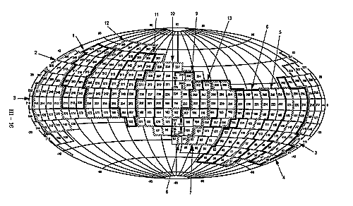
Figure III.C.1(a) Field-Group Boundaries for the
12 and 25 µm Local Destriper Processing in Equatorial Coordinates larger largest |
 | < 50°
sky were processed differently through the local destriper
from the fields covering the || > 50° sky.
For the high-ecliptic-latitude sky, parameters were derived
for each detector within a 12.5° field independent of
the surrounding fields. This was possible due to the large number of
crossing scans within any given field at the higher latitudes.
For fields nearer the ecliptic plane, the scans were nearly parallel
and therefore did not have as much crossing information to
reduce the effect of the residual zodiacal emission.
Processing these fields independently of surrounding fields would
have resulted in poorer quality images and the loss of the ability to mosaic.
To take advantage of the surrounding information, several 12.5°
fields (20-40) were concatonated into one large field, known
as a field-group, and
sent through the local destriper. Parameters were derived, as
before, for each scan segment within a field-group. Even though a
single IRAS scan crossed several
ISSA 12.5° fields which make up a field-group,
the different scan segments were treated separately
when deriving local destripe parameters.
Including information from adjacent fields
forced agreement in the overlap regions. The overlap from the
adjacent fields and from higher latitude fields where there are
crossing scans allowed a better destriping result. For the 12 µm and
25 µm images, the sky was divided into 13 field-groups.
A list of ISSA fields that make up each field-group is
found in Tables III.C.1(a) and
III.C.1(b).
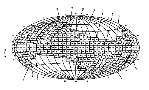
Field-groups were defined differently for 60 µm and 100 µm
as shown in Figures III.C.1(a) and
III.C.1(b). Some field-groups
overlapped to preserve integrity at field boundaries.
By using these large fields as input to the local destriper, most
images remain mosaickable. Boundary discrepancies,
on the order of one to two MJy sr-1 at
60 µm and three to five MJy sr-1 at 100 µm,
remain near the Galactic plane and
where the higher latitude fields join the field-groups.
| < 50°
sky were processed differently through the local destriper
from the fields covering the || > 50° sky.
For the high-ecliptic-latitude sky, parameters were derived
for each detector within a 12.5° field independent of
the surrounding fields. This was possible due to the large number of
crossing scans within any given field at the higher latitudes.
For fields nearer the ecliptic plane, the scans were nearly parallel
and therefore did not have as much crossing information to
reduce the effect of the residual zodiacal emission.
Processing these fields independently of surrounding fields would
have resulted in poorer quality images and the loss of the ability to mosaic.
To take advantage of the surrounding information, several 12.5°
fields (20-40) were concatonated into one large field, known
as a field-group, and
sent through the local destriper. Parameters were derived, as
before, for each scan segment within a field-group. Even though a
single IRAS scan crossed several
ISSA 12.5° fields which make up a field-group,
the different scan segments were treated separately
when deriving local destripe parameters.
Including information from adjacent fields
forced agreement in the overlap regions. The overlap from the
adjacent fields and from higher latitude fields where there are
crossing scans allowed a better destriping result. For the 12 µm and
25 µm images, the sky was divided into 13 field-groups.
A list of ISSA fields that make up each field-group is
found in Tables III.C.1(a) and
III.C.1(b).
Field-groups were defined differently for 60 µm and 100 µm
as shown in Figures III.C.1(a) and
III.C.1(b). Some field-groups
overlapped to preserve integrity at field boundaries.
By using these large fields as input to the local destriper, most
images remain mosaickable. Boundary discrepancies,
on the order of one to two MJy sr-1 at
60 µm and three to five MJy sr-1 at 100 µm,
remain near the Galactic plane and
where the higher latitude fields join the field-groups.
|
|
|
Figure III.C.1(b) Field-Group Boundaries for the
60 and 100 µm Local Destriper Processing in Equatorial Coordinates larger largest |
| Field-Group | ISSA and ISSA Reject Fields |
|---|---|
| 1 | 139 172 173 174 175 208 209 210 211 244 245 246 247 280 281 282 283 314 315 316 317 345 346 347 348 372 373 374 375 395 |
| 2 | 108 109 139 140 141 142 143 175 176 177 178 179 211 212 213 214 215 247 248 249 250 251 283 284 285 286 317 318 319 320 348 349 350 375 |
| 3 | 54 55 80 81 82 109 110 111 112 143 144 145 146 179 180 181 182 215 216 217 218 251 252 253 254 286 287 288 289 290 320 321 322 323 350 351 352 353 354 |
| 4 | 56 57 58 59 82 83 84 85 86 113 114 115 116 147 148 149 150 183 184 185 186 219 220 221 222 255 256 257 258 290 291 292 323 |
| 5 | 37 38 58 59 60 61 85 86 87 88 116 117 118 119
150 151 152 153 186 187 188 189 222 223 224 225 258 259 260 261 |
| 6 | 37 38 39 40 60 61 62 63 87 88 89 90 118
119 120 121 152 153 154 155 188 189 190 191 224 225 226 227 260 261 262 263 |
| 7 | 40 63 64 65 66 90 91 92 93 121 122 123 124 155 156 157 158 191 192 193 227 228 229 230 263 264 265 266 298 299 300 331 332 |
| 8 | 66 67 93 94 95 96 124 125 126 127 128 158 159 160 161 162
194 195 196 197 198 230 231 232 233 234 266 267 268 269 270 300 301 302 303 304 332 333 334 335 364 |
| 9 | 95 96 97 127 128 129 130 131 162 163 164 165 166 198 199 200 201 202 234 235 236 237 238 270 271 272 273 304 305 306 307 308 335 336 337 338 339 364 |
| 10 | 100 130 131 132 165 166 167 168 201 202 203 204 237 238 239 240 272 273 274 275 276 307 308 309 310 338 339 340 341 364 367 368 |
| 11 | 169 170 171 172 205 206 207 208 241 242 243 244 277 278 279 280 311 312 313 314 342 343 344 345 369 370 371 372 392 393 394 395 |
C.4 Image Assembly
Once the zodiacal foreground and detector stripes were removed, the position-ordered detector data were projected and binned into an image. This process utilized a gnomonic projection to convert sky position into image line and sample values for each detector. After all scans were binned for a given field into separate HCON images, the co-added images were created. Data in the positions of known asteroids were removed from the individual HCON data stream prior to creating the co-added images. All images were then visually inspected for anomalies.The gnomonic projection used in the ISSA was the same as that used in the SkyFlux images (Main Supplement §X.D.2.a). It produced a geometric projection of the celestial sphere onto a tangent plane from a center of projection at the center of the sphere. Each individual field has its own tangent projection plane with the tangent point at the center of the field. The ISSA binning algorithm placed the detector intensity value into each pixel within a 2' radius of the actual detector position on the image. No adjustment was made for scan direction and there was no weighting based on the spatial responsivity function of the detectors. The resultant point spread functions are discussed in §IV.C. Cumulative information per pixel was kept for each HCON, including the sum of intensities, counts and sum of intensities squared. After all scans were binned, a final intensity image at each wavelength was made by using the simple mean intensity at each pixel. An image of the standard deviation was also calculated.
The number of data points per pixel varies depending on sky coverage. For the sky covered by two HCONs, a typical average count per pixel is 10-14 depending on band with a maximum count of around 16. For the sky covered by three HCONs, a typical average count per pixel is 15-20 depending on band with a maximum count of around 30. These counts increase for fields at higher ecliptic latitudes. At the north ecliptic pole a typical average is 25-50 with a maximum of around 65-70.
An attempt was made to automate the rejection of nonconfirming objects prior to co-addition by examining the flux distribution within a single pixel. In principle, a nonconfirming object would differ sufficiently from the overall distribution such that it could be recognized and rejected by setting a simple threshold based on the flux distribution. However, the distribution of brightness among scans was so varied, especially around point sources, that nonconfirming objects could not be rejected without setting the threshold to one or two sigma. In addition, asteroids are only 2.1 sigma from the mean in the part of the sky covered by three HCONs. Therefore, no confirmation algorithm was implemented.
Since the population distribution was not useful in separating out artifacts, the noise images (§I.C) were considered to be of minimal utility and therefore were not released.
| Field | Field | Field |
|---|---|---|
| 115 | 164 | 203 |
| 116 | 166* | 204 |
| 117 | 167* | 216 |
| 118 | 180 | 217 |
| 119 | 181 | 218 |
| 120 | 182 | 219 |
| 121 | 183 | 220 |
| 128* | 184 | 221 |
| 129* | 185 | 232 |
| 145 | 190 | 233 |
| 146 | 191 | 234 |
| 147 | 192 | 235 |
| 148 | 193 | 236 |
| 149 | 194 | 252 |
| 150 | 195 | 253 |
| 153 | 196 | 254 |
| 154 | 197 | 255 |
| 155 | 198 | 272 |
| 159 | 199 | 282 |
| 160 | 200 | 283 |
| 162 | 201 | 316 |
| 163 | 202 | 317 |
Data in the position of known asteroids were
removed only from the co-added images. A list
was obtained from the IRAS Asteroid and Comet Survey (Matson 1986).
This
database provided detector and sighting times. The actual window
of data removed depended on the duration
of the sighting on a detector. A pad of one second prior and two
seconds after the given sighting was used to account for the
effects of the convolution filter used in creating the compressed,
time-ordered detector data.
Comet tails and trails were not removed from the co-added images.
Most comet trails appear near the ecliptic plane where there
remains a difference in the residual zodiacal foreground between
HCONs primarily due to the zodiacal bands.
Given the different background levels for each HCON, the removal of
comet trails in this region from the individual HCON data prior
to co-addition would result in undesirable streaks in the co-added image
along the paths of the clipped comet trails.
No fields in the || > 50°
sky are affected by comet trails.
The comet tail of IRAS-Araki-Alcock is seen in fields 416
and 418. A list of fields affected by comet trails is found in
Table III.C.2.
Figure III.C.2 shows the comet trails for different HCONs.
Note that all but four fields (128, 129, 166 and 167)
are from the ISSA Reject Set.
A list of trail positions is found in Sykes and Walker 1992.
*ISSA fields NOT in the ISSA Reject Set.
|
|
|
Figure III.C.2 Known Comet Trails as Seen by IRAS
Plotted in Equatorial Coordinates larger largest |
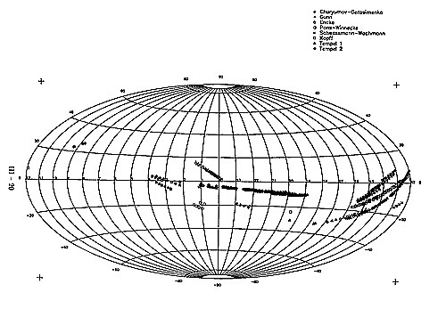
Table III.C.3 lists the position and corresponding
ISSA field affected by planets.
Jupiter was specifically avoided during the IRAS mission due
to the stength of its infrared radiation.
Mars was not viewed by IRAS due to a coincidence between its motion
and the timing of survey observations near its location.
Venus and Mercury were not scanned due to their proximity to
the Sun. Pluto is too faint to be detectable in the ISSA data
(Aumann and Walker 1987).
| Planet | Field | RA | DEC |
|---|---|---|---|
| Uranus | 150 | 16h10m36.9s | -21d02m21s |
| Saturn | 183 | 13h45m18.2s | -08d13m07s |
| Neptune | 152 | 17h43m03.5s | -22d13m57s |
| Neptune | 153 | 17h54m20.9s | -22d11m59s |