Computing Scan Coverage

Author:: Serge Monkewitz

	Contents
	What is a Scan? Scan coverage Brute force algorithm BSP Algorithm Coarse subdivision BSP trees Computing scan coverage with a BSP tree Scan coverage across small areas

What is a Scan?

A scan, in the sense understood by the WAX software, is a convex polygon on the unit-sphere, with four unit vector corners and four great circle edges. This quadrilateral approximates an observed area on the sky, an area for which raw image data is available and has been used for apparition extraction.

This page describes algorithms which determine how many such scans cover a particular position on the sky - a quantity which roughly indicates the expected number of apparitions of a single astronomical source located at that position, assuming an ideal instrument and observation conditions.

A scan $s_i$ has four corners $c_{i0}, c_{i1}, c_{i2}, c_{i3} \in \Re^3$ , with edges linking corners 0 and 1, 1 and 2, 2 and 3, and 3 and 0. Each great circle edge can be specified with a single vector perpendicular to the plane passing through the origin and both edge vertices :

$n_{i0} = \frac{c_{i0} \wedge c_{i1}}{\Vert c_{i0} \wedge c_{i1} \Vert},\; n_{i1} = \frac{c_{i1} \wedge c_{i2}}{\Vert c_{i1} \wedge c_{i2} \Vert}.\; n_{i2} = \frac{c_{i2} \wedge c_{i3}}{\Vert c_{i2} \wedge c_{i3} \Vert},\; n_{i3} = \frac{c_{i3} \wedge c_{i0}}{\Vert c_{i3} \wedge c_{i0} \Vert}$

The corners are numbered such that they appear in counter-clockwise order when viewed from outside the unit-sphere in a right handed coordinate system.

Scan coverage

The scan coverage for a position (unit-vector) $p$

is defined as the number of scans covering $p$

For $p$ to lay inside a scan $s_i$ , it must satisfy the following four conditions :

$p \cdot n_{i0} \geq 0,\; p \cdot n_{i1} \geq 0,\; p \cdot n_{i2} \geq 0,\; p \cdot n_{i3} \geq 0$

that is, $p$ must lay inside each of the edge planes.

Brute force algorithm

The obvious method of determining scan coverage for a position $p$

is to perform the test above for each existing scan.

Since the databases being processed involve apparitions from up to 70000 scans, this would involve performing between 70000 and 280000 dot products and comparisons to determine the scan coverage of a single position.

Because scan coverage is likely to be computed for the position of every group generated by WAX, this algorithm is unacceptable.

BSP Algorithm

The BSP algorithm uses two forms of spatial subdivision, both of which lower the number of dot-products and comparisons required to determine scan-coverage for any given position.

Coarse subdivision

First of all, the sky is divided into 256 declination bands (each of height $\frac{\pi}{256}$ radians). Each band is further subdivided into equal width lanes, with a minimum lane width of 0.3 degrees. This subdivision scheme is essentially identical to the one used for apparitions (see Lane Subdivision), but is performed on scans and on a much coarser scale.

If a list of overlapping scans were stored for each lane, this coarse subdivision scheme would already drastically reduce the number of coverage tests required for a position. However, there are datasets which contain clusters of more than 3000 scans, stacked virtually on top of eachother. Simple binning as described would still incur a cost of up to 12000 dot products per position for these cases.

Therefore, instead of storing a list of overlapping scans for each lane, the overlapping scans are used to generate a Binary Space Partitioning (BSP) tree. This tree is stored for each lane in every band, and is used for all coverage computations.

BSP trees

A BSP tree is generated from a set of convex polygons by recursively splitting the set against edge planes. Note that existing algorithms for clipping polygons in 2-D can easily be extended to work with polygons on the surface of the unit-sphere.

Let $P$ be the set of polygons corresponding to scans.

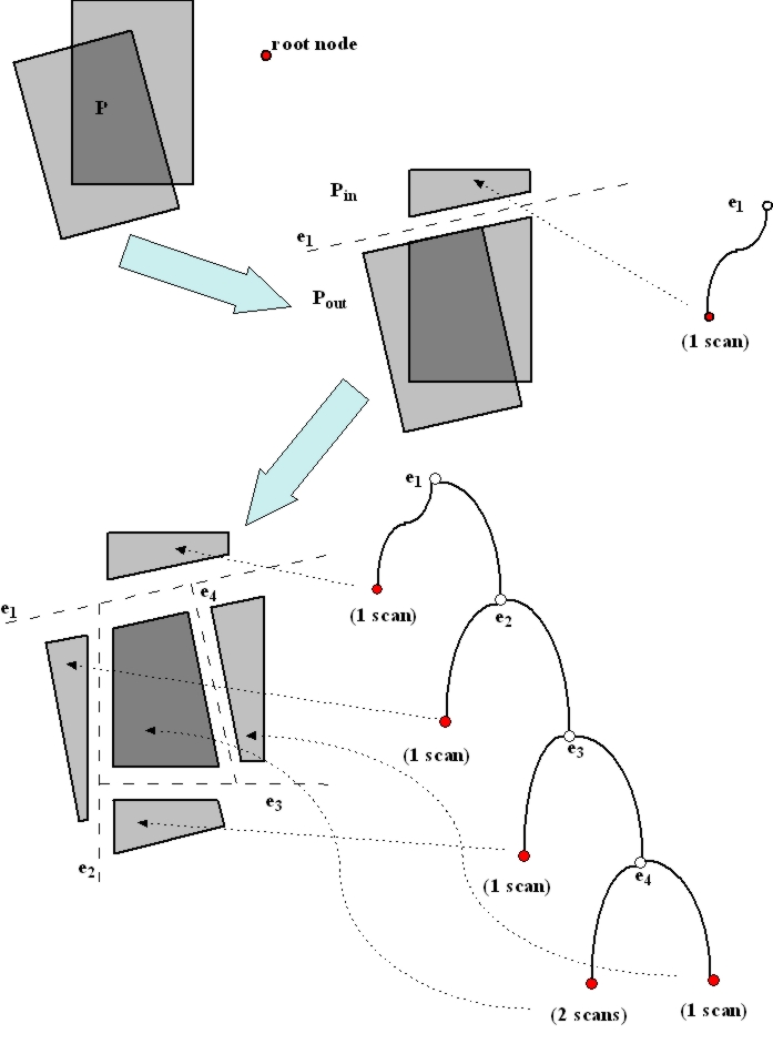
From a polygon in , take an as yet unconsidered edge plane and use it to split into two polygon sets, one containing polygons completely inside the chosen edge plane, $P_{\rm in}$ , the other containing polygons completely outside, $P_{\rm out}$ . Polygons straddling the edge plane are themselves split into an inside and outside polygon (using the aforementioned clipping algorithms).
If $P_{\rm in}$ is non-empty and contains a polygon with an as yet unconsidered edge plane, feed $P_{\rm in}$ to step 1. Otherwise, store the number of polygons in $P_{\rm in}$ . Then continue with step 3.
If $P_{\rm out}$ is non-empty and contains a polygon with an as yet unconsidered edge plane, feed $P_{\rm out}$ to step 1. Otherwise, store the number of polygons in $P_{\rm out}$ .

The process, illustrated below, produces a binary tree in depth first order, where nodes correspond to splitting planes and leaves are convex polygons inside of which scan coverage is constant (no leaf contains a scan edge).

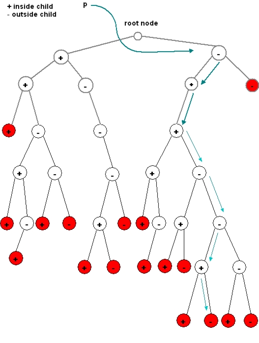
Computing scan coverage with a BSP tree

Computing the scan coverage for a position $p$

is equivalent to finding the BSP tree leaf containing $p$

. This is easily done, starting with a current node equal to the root node of the tree :

Using the splitting plane normal of the current node, determine whether belongs to the inside or outside child of the current node :
- $p \cdot n \geq 0 \Leftrightarrow p$ belongs to the inside child
- Otherwise ( $p \cdot n < 0$ ), belongs to the outside child
If the child containing is a node, set the current node to equal the child and continue with step 1.
Otherwise, the child containing is a leaf. Since scan coverage is constant inside each leaf, the scan coverage for has been found and the computation is complete.

This process is illustrated below, with empty leaves (those with 0 scan coverage) omitted from the diagram.

The ascent of the tree will involve a number of nodes no greater than the maximum tree depth. The worst cases encountered in practice (stacks of 1500 to 3500 scans) result in tree depths between 12 and 40. Since one dot product is performed for each node visited in the BSP tree, the algorithm performs at most 40 vector dot products for a scan coverage computation (as opposed to between 1500 and 14000).

Scan coverage across small areas

Similarly, the minimum and maximum scan coverage of the positions inside a given search area can be found by finding the minimum and maximum scan coverage of the leaves intersecting the search area.

The WAX software currently only supports small circular search regions, specified as a search region center, $p$ , and a search radius, $r_s$ . A position $v$ is inside the area if and only if $\cos{r_s} \leq v \cdot p$ .

Finding the leaves intersecting the search area is accomplished as follows, starting with a current node equal to the root node of the tree :

Using the splitting plane normal of the current node, determine whether the search area intersects the inside and outside children of the current node.
If , then the search region touches the inside child :
- If the inside child is a node, set the current node to equal the child and continue with step 1.
- Otherwise, the inside child is a leaf. Compare the scan coverage for the leaf to the minimum and maximum scan coverage values found so far and update them if necessary.
if , then the search region touches the outside child :
- If the outside child is a node, set the current node to equal the child and continue with step 1.
- Otherwise, the outside child is a leaf. Compare the scan coverage for the leaf to the minimum and maximum scan coverage values found so far and update them if necessary.

Picking a search radius $r_s = 0$ will produce a minimum and maximum scan coverage equal to the scan coverage for $p$ .

Generated on Thu Oct 21 13:19:39 2004 for WAX Version 2.1 by

1.3.8