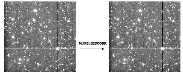
The InSb arrays suffered from an effect known as “muxbleed” (for more information on this effect see Section 7.2.2). This was thought to be a result of operating the arrays at unusually cold temperatures. When a bright source was read out, the cold electronics did not return to their quiescent state for a considerable length of time. The result was ghosting along the pixel readout channels, sometimes referred to as “ant trails” (Figure 5.8). The effect was easily noticeable against a low background (such as a dark current measurement), and could extend the full length of the array. The muxbleed flux was not real, i.e., it was not “borrowed” from the actual source.
Figure 5.8: Before (left) and after (right) correction of pseudo-muxbleed for channel 1. Shown is a bright source within a calibration AOR and a background of sources under the muxbleed limit.
This effect was complicated. It appeared that a pixel bleeds only as a result of the light falling onto it, and not as the sum of the value of the pixel plus the bleeding from previous pixels. Since we knew the readout order of the pixels, we could start by correcting all the pixels downstream from the first pixel, and then move on to the next pixel. The exact shape of the muxbleed pattern, obtained after examining hundreds of muxbleed incidences, is summarized as a modified polynomial:
Pixel numbers were counted along the detector readout direction, starting from the muxbleed causing pixel (pixel number zero). The muxbleed pattern appeared to be independent of readout channel, Fowler sampling, etc. Furthermore, the pattern seemed to be applicable to both the channel 1 and channel 2 muxbleed, with a slightly different scaling factor. The severity of muxbleed depended on the brightness of the bleeding pixel. Muxbleed scaling laws as a function of the bleeding pixel were obtained for channels 1 and 2. They are
(5.11)
where
x = log10(bleeding pixel intensity in DN).
(5.12)
For channel 1, A = 0.6342, B = 5.1440, and C = 0.5164. For channel 2, A = 0.3070, B = 4.9320, and C = 0.4621. Both the scale factors and the muxbleed pattern were fixed for all the pixels in a given array. Muxbleed from triggering pixels with brightnesses below 10,000 DN was not corrected, because the corrections in these cases would be just a few times the read noise. Muxbleed was also not corrected in the subarray observations.
Observers should note that calibration darks were not muxbleed corrected. Muxbleed occurred in these images due to the presence of hot pixels. However, this occurred equally both in the darks and in the science frames and was found to subtract noiselessly from the science data. Thus, any dark frame muxbleed was simply considered a feature of the darks.
Note that the muxbleed correction described here did not always correct 100% of the muxbleed effect. Muxbleed was not present in the warm mission data due to the higher operating temperature and voltages.
Each IRAC array was read out through four separate channels. The pixels read out by these channels were arranged vertically, and repeated every four columns. Small drifts in the bias levels of these readouts, particularly relative to the calibration dark data, could produce a vertical striping called the “jailbar” effect. This was mostly noticeable in very low background conditions. This was corrected by adding to the individual readout channels a common mean offset. For any image, the flux in a pixel was assumed to be
(5.13)
where i is the readout channel number (1-4), j is the row number, A is the detected intensity in DN, S is the incident source flux (celestial background + objects), B is a constant offset in the frame, DC is the standard calibration dark, and DO is the dark offset. The first dark varied on a pixel by pixel basis, whereas the offsets were assumed to vary on a readout channel basis. The correction step determined a common background level, equal to the mean of the backgrounds in the four readout channels. These were determined by a robust mean estimator function M
Mi= MeanEstimator(Si,0…Si,n)
(5.14)
The corrected image (post dark-subtraction) was then
.
(5.15)
5.1.13 fowlinearize (detector linearization)
Like most detectors, the IRAC arrays were non-linear near full-well capacity. The number of read-out DN was not proportional to the total number of incident photons; its rate of increase with fluence decreased as the fluence increased. In IRAC, if fluxes were at levels above half full-well (typically 20000–30000 DN in the raw data), they could be non-linear by several percent. During processing the raw data were linearized on a pixel-by-pixel basis using a model derived from ground-based test data and re-verified in flight. The software module that did this was called fowlinearize. fowlinearize worked by applying a correction to each pixel based on the number of DN, the frame time, and the linearity solution. For channels 1, 2, and 4, we used a quadratic solution, i.e., we modeled the detector response as
DNobs = kmt – Ak2t2
(5.16)
where k is the source rate (linear DN/second), and m and A are linearity fit coefficients. The linearization solution to the above quadratic model is:
(5.17)
where
,
(5.18)
and , n is the Fowler number, w is the wait period, td is the delay from reset to first readout, and tc is the clock readout time. The above expression for L is the correction required to account for multi-sampling. This was required because the multi-sampling resulted in the apparent time spent integrating not actually being equal to the real time spent collecting photons. Note that td is the time between the reset and the first readout of the pixel. For channel 3, we used a cubic linearization model:
DNobs = Ckt3 + Akt2 + kmt
(5.19)
For the cubic model, the solution was derived via a numerical inversion.
5.1.14 bgmodel (zodiacal background estimation)
For this module, a spacecraft-centric model of the celestial background was developed. For each image, the zodiacal background was estimated (a constant for the entire frame) based on the pointing and time that the data were taken. This value was written to the header keyword ZODY_EST in units of MJy/sr. The zodiacal background was also estimated for the subtracted skydark (see next module) and placed in the header keyword SKYDRKZB.
5.1.15 Dark Subtraction II: skydarksub (sky “delta-dark” subtraction)
This module, the second part of dark subtraction, strongly resembled traditional ground-based data reduction techniques for infrared data. Since IRAC did not use the shutter for its dark measurement, a pre-selected region of low zodiacal background in the north ecliptic cap was observed in order to create a skydark (see Section 4.1). At least twice during each campaign a library of skydarks of all Fowler numbers and frame times were observed, reduced, and created by the calibration pipeline. The skydarks had the appropriate labdark subtracted in their DARKCAL pipeline and were therefore a “delta-dark.” These skydarks were then subtracted from the data in the pipeline within this module, based on the exposure time, channel, and the time of the observation. Note that there was a problem with the skydark subtraction from the 58th frame in the subarray observations which left the background level in that frame different from the rest. While this should not affect photometric measurements, users may want to choose to leave the 58th subarray frames out from their analysis.
5.1.16 flatap (flat-fielding)
Like all imaging detectors, each of the IRAC pixels had an individual response function (i.e., DN/incident photon conversion). To account for this pixel-to-pixel responsivity variation, each IRAC image was divided by a map of these variations, called a flat-field. See also Section 4.2 and 7.1.2.
Observations were taken of pre-selected regions of high-zodiacal background with relatively low stellar content located in the ecliptic plane. They were dithered frames of 100 seconds in each channel. These observations were processed in the same manner as science data and then averaged with outlier rejection. This outlier rejection included a sophisticated spatial filtering stage to reject the ever-present stars and galaxies that filled all IRAC frames of this depth. The result was a smoothed image of the already very uniform zodiacal background. This skyflat is similar to flat-fields taken during ground-based observations. The flat-fields were then normalized to one, using a median, and excluding a 3-pixel wide border at the edges of the image. A central area was used for calculating the normalizing median in the cryogenic mission, whereas the whole array was used in the warm mission (excluding the border mentioned above). The flat-field calibration pipeline produced a library of the flat-fields throughout each campaign as a flat-field was taken at the beginning and end of an observing campaign. We found that there was no difference in flat-fields from campaign to campaign, so a “superskyflat,” composed of five full years of data and therefore of very high SNR, was used for processing science data in the BCD pipeline. A separate superskyflat was created for cryogenic and warm data. It should be noted that this flat-field was generated from a very red target, i.e., the zodiacal background. There was considerable evidence for a spatially-dependent color term in the IRAC calibration (which was roughly a quadratic polynomial function across the array). Objects that have color temperatures radically different from the zodiacal background require an additional multiplicative correction of order 5% – 10%. This was not treated by the flat-fielding stage. See Section 4.5 for more details.
Software module flatap applied the flats generated by the calibration server. This operation was equivalent to division by the flat.

 ,
,