2.10.4         Spectroscopic Sensitivity Correction for Bright Sources

The PSSC and PSSCS as calculated above and shown in the sensitivity curves assume that the target is in the faint source limit.  That is, the shot noise from the source is negligible compared with the other sources of noise described above.  Conversely, Figure 2.20 shows the approximate flux density (the median flux density averaged over the whole wavelength response of each module) at which a target’s shot noise dominates over the other sources of noise (sky background + dark current + read noise), as a function of exposure duration for each of the IRS modules.  Thus, Figure 2.20 can be used to determine whether a target object of known infrared flux density corresponds more appropriately to the “Bright Source Limit” (BSL).

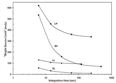
The low-resolution modules rapidly reach an asymptotic BSL in a few tens of seconds of integration time, whereas the high-resolution modules take longer to reach this plateau.  Sources that have flux densities which lie below the curves plotted in Figure 2.20 for a given integration time are in the faint-source limit (i.e., they are background or read-noise limited), whereas sources that have flux densities which place them above the line for a given module have signal-to-noise ratios (S/N) that are dominated by the source flux density.  Knowledge of the regime in which a source lies is crucial to calculating a realistic S/N estimate.  Note that for all allowed AOT integration times of the low resolution modules, sources brighter than 130 mJy will always be source-dominated.  For all allowed AOT integration times of the high resolution modules, sources brighter than 620 mJy will always be source-dominated.

In this section, we provide a simple scaling rule that allows the original estimate of the signal-to-noise ratio for faint sources obtained through the use of Figure 2.15 through Figure 2.18 to be corrected for the contribution of the shot noise from a bright source.  Consider, for example, a continuum source with a known 8 micron flux density of 250 mJy.  To estimate the S/N of this source in the SL module for an integration time of 14 sec, we first consider the PSSC for SL at this wavelength (i.e., the faint source limit case).  Inspection of Figure 2.15 shows that at 8 microns, the 1  PSSC is 0.7 mJy (in the LOW background case).  If we were to (incorrectly) assume that the source itself contributed no noise, then we would estimate the signal-to-noise ratio (S/N)_faint = (250/0.7) = 357.  However, we notice from Figure 2.20 that in SL for a 14 sec integration time, the Bright Source Limit (BSL) = 26.5 mJy.  Thus, the 250 mJy target exceeds the BSL by a factor of ~9.4.  We can now estimate a more realistic S/N for the source by using the simple scaling rule

Equation 2.11

Where the source and BSL fluxes are given in the same units (e.g., mJy).  In this example,

Equation 2.12

Hence, a more realistic value for the 8 micron S/N for a 250 mJy source observed for 14 sec in SL is ~110.  This procedure can be generalized for use in estimating the S/N that was obtained for observations of bright sources (both point and extended) using any of the IRS modules.

Figure 2.20:  Bright Source Limit (BSL) as a function of integration time for each of the IRS modules.  Targets with fluxes above the curves for a given integration time are source-dominated; targets with fluxes below the curves are read noise or background limited.  The plotted points on the curve for each module indicate the allowed AOT durations for that module. 

• 
• 
• 
• 
•