The LINEARIZ (“Linearization”) module corrects the ramps of IRS DCEs for the non-linear response of the detectors. In the absence of this effect, the signal of a given sample, in a particular pixel (ramp), would ideally be a linear function of time from the beginning of the DCE, or equivalently of plane (sample) number counting from the first sample of the ramp.
An empirical, one-parametric model of non-linearity relates the observed signal Sobs of a sample of a given ramp, to the ideal signal Slin that would be observed in the absence of non-linearity:
Equation 5.9
The parameter is the so-called non-linearity coefficient. In the IRS pipelines, < 0, and its absolute value is | | ~ 10-7 to 10-6 . Its units, 1/electron, are the reciprocal of the units of Slin or Sobs.
The above exponential model is used in SATCOR. A series expansion of the exponential, keeping terms up to second order, leads to the so-called quadratic model of non-linearity that is used in LINEARIZ:
Equation 5.10
The above can be solved for Slin as a function of Sobs; only one of the two quadratic solutions is valid, given the requirement that Sobs should approach Slin as α approaches 0:
Equation 5.11
The application of the above expression, given the input signal Sobs of a sample, and the non-linearity coefficient obtained from the lincal.fits calibration file, constitutes the main algorithm of the LINEARIZ module.
There are two conditions under which the module cannot correct a sample Sobs. In either case, a fatal bit is set in the output (updated) dmask.fits file for the corresponding sample.
-If Sobs is larger than a threshold for non-linearity read from the lincal.fits calibration file, the sample is deemed as “saturated beyond correctable non-linearity.” The threshold in current IRS pipelines is 280,000 electrons. IRS observations typically do not reach this threshold without also being digitally saturated. Bit # 13 is set in the dmask.fits corresponding sample.
-If Sobs> |1/4|, the solution for Slin is imaginary. In such case, it is deemed that linearity could not be applied for the particular sample. Bit # 12 is set in the corresponding dmask.fits sample.
The calibration file lincal.fits is a 3-plane cube. Its first plane contains the coefficient for each of the 16,384 pixels in IRS arrays. The same value of is used for all pixels of a given instrument channel. The second plane contains the threshold for saturation beyond correctable non-linearity, for each pixel. The third plane is the uncertainty in , also for each pixel. This uncertainty is propagated in the BCD pipeline.
The outputs of this module are lnz.fits and lnzu.fits.
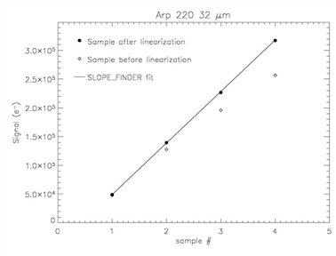
Figure 5.5 Illustration of non-linearity correction in a LL 6 second ramp for a bright source: the open rhombii are input samples, referred to as Sobs in the text; the filled circles are output samples, referred to as Slin, after the operation of LINEARIZ. The solid line is the linear fit computed by the subsequent module SLOPE_FINDER.