SPHEREx Data Explorer: Mosaic Tool
Every location in a SPHEREx image has a unique ra, dec, and
wavelength. Therefore, in order to make a mosaic that consists of
data that are all one smaller wavelength regime, you have to pull apart
individual images and reassemble them. That is what the Mosaic Tool
does. This Mosaic Tool is integrated into the
SPHEREx Data Explorer, building on core capabilities of Tables, Plots, and Images. Generic help on those capabilities
can be found in those other sections; this section is specific to the
Mosaic Tool. The first few subsections explain how the
tool works conceptually, while the later subsections provide
step-by-step instructions for running it.
Contents of page/chapter:
+Introduction
+Background
+Initiating a Process <-- Jump here
to learn more about starting a job
+Job Monitor
+Results
+Exploring Bitflags
+Saving Results
+Tips for Success
The SPHEREx Mosaic Tool combines data across multiple SPHEREx Spectral
Images to generate a mosaic that consists of a relatively narrow range
of wavelengths. For this release, the tool produces a cube with each
plane at the 102 nominal wavebands (default) or a user-specified
smaller range of the nominal wavebands. You can specify the pixel
size, but the smallest pixel size is 6.15 arcsec (the nominal pixel
size). You can specify the size of the mosaic, but the largest mosaic
is 5x5 degrees.
Since the mosaic tool produces a cube where each plane is a different
mosaic, you can use the extraction tools to very
quickly drill through the cube to generate a spectrum-like product.
The drill extraction tool is NOT THE SAME as the spectrophotometry
tool! The drill extraction tool provides a quick look through the
cube, intended for exploratory use.
Cukierman et al. (2026) describes SPHEREx map-making methodologies in
general, and the Explanatory Supplement, available from the SPHEREx Mission Page, describes this specific Mosaic Tool in more detail.
describes SPHEREx map-making methodologies in
general, and the Explanatory Supplement, available from the SPHEREx Mission Page, describes this specific Mosaic Tool in more detail.
In terms of a high-level summary of the algorithm, this is Figure 6
from Cukierman et al. (2026):

The three columns denote three stages
of coaddition of a mosaic. The first column denotes the extraction of
a spectral channel centered on 3.913 microns from a single exposure.
That same spectral channel extracted from 8 exposures is in the second
column, and that same spectral channel extracted from 446 exposures is
in the third column. Note that each stripe extracted from a single
image has a range of wavelengths included (third row), which can
result in striped artifacts in the final mosaic until there are enough
data built up such that there is enough overlap as to average out
these artifacts. Some parts of the sky still do not have enough data
yet to even create complete mosaics at a given band; as the mission
continues, these gaps will be filled in over time.
Currently, the tool only uses images from the all-sky survey. Later
versions will include images from the deep field.
The screen from which you initiate a spectrophotometry process looks
very much like the Spectral Image Search
or the Spectrophotometry Tool,
but it is different.

Just like in a Spectral Image
Search, you have a HiPS
image loaded that takes up most of the browser area. Overlaid on
top of the HiPS image, there is a MOC indicating the sky coverage for
the data currently available in the archive, and one for the deep
fields coverage. As you zoom in, the shaded regions become more
transparent, or you can change them in the layers pop-up.
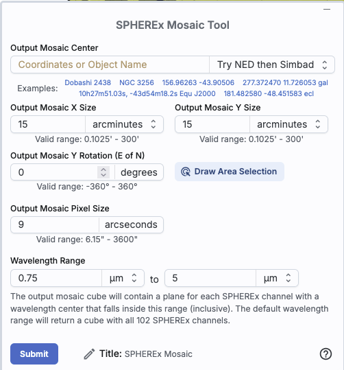
Parameters
|
Just like in all the other search windows, you need to specify a target for the mosaic; please see
that section for details of how to do that (what syntax, coordinate
systems, etc.). As soon as you put in a position, it will draw a box
at the location you specify on the HiPS image. You can initially
select a position, or refine a position, by clicking on the HiPS
image.
Next, you need to specify the size of the output mosaic; the default
is 15x15 arcmin. It need not be a square; it can be a rectangle.
Specify the units first, and then the number. (If you put in the
number first and then change the units, it will convert the number.)
You can request tiny mosaics (one pixel, 6.15 arcsec), or large
mosaics, up to 5 degrees on a side. As you update the numbers here,
the box it has drawn on the HiPS image dynamically updates.
You can specify the mosaic rotation in degrees east of north.
You can also draw an area selection on the HiPS image.
You need to specify the output mosaic pixel size -- the smallest
available is 6.15", the native size of SPHEREx pixels, and the
largest is 3600 arcsec. The default is 9 arcsec.
You need to specify the wavelength range you want; the default is the
full 0.75-5 microns. The bandpasses the tool uses is the default 102
SPHEREx nominal channels.
And, just like in a Spectral Image Search or a spectrophotometry jobs,
these mosaic jobs are managed in the Job Monitor. If you are submitting a
lot of jobs, keeping track of which job is which in list in the Job
Monitor can be difficult. Using the "Title" field near the bottom of
the mosaic window, you can change the title by which the search will
be listed in the Job Monitor. You don't have to change it from the
default to be able to submit jobs, however. (Once you change it,
though, all subsequent jobs you make will still have that same title
unless you change it each time.)
|
Any mosaic job, even a point source with minimal wavelength coverage,
takes measurable time. Therefore, you should send the job to the Job Monitor.

Click on "Send to Background", and the job monitor will take over
management of the job; you can then continue to work in the tool while
you wait. See the Job Monitor section
of the Downloads chapter for more information.
The length of time for the job to run should be much faster than the
spectrophotometry tool, but it will be proportional to the number of
images it has to combine, and the number of pixels it has to contend
with (smaller pixels take longer), to make your final mosaic.
After a mosaic job finishes in the Job Monitor, click on
the icon that matches that in the "Results" tab  to display the results of this job in the
tool.
to display the results of this job in the
tool.
Here are the results of a mosaic run:

Note that:
- All I have done in this session is create a mosaic, so I have only
one window pane in the results tab, and it's just an image, not a list
of anything.
- The mosaic comes up as a pinned image, in the "Mosaic/Pinned
Image" tab.
- All of the other tabs ("Data", "Coverage", "Details", and "Active
Chart") are empty. This is normal since all I have done is create a
mosaic.
- In the resultant mosaic, there are 3 HDUs: IMAGE, NHITS, FLAGS.
(See below for more information.) Each HDU has 102 planes, one for
each of the nominal SPHEREx bandpasses.
The "IMAGE" HDU is the final product, in units of MJy/sr. The "NHITS"
HDU is the number of input images that hit that pixel on the sky. The
"FLAGS" is the aggregate bitflags -- selected flags are propagated to
the output via bitwise or accumulation. These are overflow, outlier,
and source. See the Explanatory Supplement, available from the SPHEREx Mission Page, for more information.

This is the result of a mosaic run after a Spectral Image
Search. After this seasrch, all the tabs are populated, largely with
results of the Image Search -- "Spectral
Images" on the left and "Data", "Coverage", "Details", and "Active
Chart" are all populated on the right, as well as "Mosaic/Pinned
Image" (which is where the mosaic appears. Based on
this search, we know that 237 individual exposures went into this
mosaic. Even with 237 individual exposures, not every wavelength is
available yet for this part of the sky -- a few planes show missing
coverage:


This is the result of a mosaic run, along with a Spectral
Image search and a spectrophotometry run. Since, by default, all the
images are linked together, if you're zoomed in on the tiny thumbnails
that are designed to help you assess the points from the
spectrophotometry, then the mosaic is also zoomed in very close. To
see the whole mosaic, you have to zoom out, as seen here, and then the
thumbnails become tiny. You can unlock the images if you want; see the
Visualization chapter.
You can use this tool to explore what flags are set in the
final product of the mosaic calculation.
This tool can automatically overlay the masks.
As described in the Visualization
chapter, you can control the layers that are shown on your
images. At the bottom of the layers pop-up, you can enable the mask
layer. When you do this, you only have three bitmasks available --
overflow (1), outlier (19), and source (21). Turn on overflow and
outlier, but leave off source. You'll be left with
color-coded indications of which pixels might be problematic:

The only way to save the results from a mosaic run is from the image
toolbar -- go to the tools dropdown:  and pick save
  . See this
chapter for more information.
. See this
chapter for more information.
⚠ Tips and
Troubleshooting
- The Job Monitor is supposed to hold on to your jobs for 14 days,
but in testing we have found some transient gremlins suggesting that
(a) you should download the data as soon as you can; (b) logging in
before submitting your jobs (and before attempting to download the
results) seems to keep the gremlins at bay for longer.
- IRSA tends to have scheduled blocktimes every other Tuesday
morning Pacific time. Those blocktimes may take down our servers and
terminate running jobs and/or lose old jobs. We are working on ways to
ameliorate this, but, again, it's probably wise to download your data
as soon as possible.
In this section, we have tried to collect all of the most important
tips for success in using this tool. You should also consult the
Explanatory Supplement on the SPHEREx Mission Page.
- Runtime 1: The more frames the tool has to work
through, the longer the process will take. Specifically because of
this, the initial version of this tool does NOT include the frames in
the Deep Field that are specifically tagged "Deep Field" frames. You
can still make mosaics in that part of the sky; they just will have a
'normal' number of frames (e.g., comparable to portions of the sky
right outside of the Deep Field). If you ask for a source relatively
close to the ecliptic poles, where there might be at least one image
per orbit, it will take a long time for the tool to work through all
the images. If you ask for a source near the ecliptic plane, where
there are fewer images, the process will complete relatively quickly.
- Runtime 2: The more pixels the tool has to deal
with, the longer it takes. If you ask for 6 arcsecond pixels and a 5x5
degree field, it will take longer than if you ask for 15 arcsecond
pixels and a 1x1 degree field.
- Even though there has been enough mission elapsed time to
nominally cover the whole sky twice, there are still parts of the sky
where complete data in particular bands has not yet been aquired. Gaps
may be present in certain wavelength planes in mosaics you generate.
- Especially in regions of the sky with fewer available frames,
there may very well be stripe artifacts, particularly in regions
overlapping with terrestrial emission. See Cukierman et al. (2026), and the Explanatory Supplement, available from the SPHEREx Mission Page.
- Throttles: To allow computing resources to be
shared fairly among all users, there are built-in throttles.
You are currently allowed a maximum of two mosaic jobs
running simultaneously. Additional jobs will be queued and run when
resources are available.
- Since the mosaic tool produces a cube where each plane is a different
mosaic, you can use the extraction tools to very
quickly drill through the cube to generate a spectrum-like product.
The drill extraction tool is NOT THE SAME as the spectrophotometry
tool! The drill extraction tool provides a quick look through the
cube, intended for exploratory use.