|
Warm IRAC Image Characteristics
(last update October 23, 2015)
This page discusses significant characteristics of data taken with the warm IRAC instrument. Generally, IRAC continues to operate in the same manner as it did when cryogenically cooled. However, there are some differences which are outlined in greater detail here. Users are advised to study the data caveats page and in particular the Warm Spitzer Observer's Manual (SOM). The Warm SOM has been updated to reflect new information regarding the operation and characteristics of the warm IRAC instrument. Additional information is presented here for emphasis, or as an update to the information in the SOM.
We have recently determined the final calibration for warm IRAC data. The SSC is currently in the process of
reprocessing the warm science data with the latest calibration and pipeline. Processing version S19.2 contains
the final calibration while S19.1 is the previous version of the pipeline. Key features of the S19.2 processing
are a flux calibration on the same system as the final cryogenic calibration and a 5th order distortion solution.
The absolute flux calibration now has an uncertainty of ~2% and the residual distortion is < 30 milliarcseconds.
We are in the process of reprocessing all existing warm IRAC data with version S19.2. The reprocessing is being
done on the most recent campaigns first and working backward in time. We estimate that it will take approximately one year to finish the reprocessing.
1. Transition Period from Cold to Warm Operations (Temperatures and Voltage Setpoints)
On May 15, 2009 Spitzer depleted the last of its cryogen. What followed was a multi-month phase during which the
telescope and instrument slowly warmed to their new equilibrium temperature. At the same time, numerous changes
were made to IRAC in order to improve its performance at the new temperature. It is important to understand this,
because the calibration of IRAC (the specific files and conversions used), as well as its calibration accuracy,
changed several times. Any user working with data taken between May 15 and September 18, 2009 must be aware of
these issues. Data products supplied by the SSC are calibrated with the best calibration available at the time of
processing, and most users should not need to apply any additional corrections. However, users must be aware that
they should not interchange calibration data within this time period, or with that from the cryogenic mission. Note
that data taken between 18 June 2009 and 18 September 2009 are less well calibrated than data taken after 18 September 2009
due to the amount of calibration data available and the fact that the calibration was slowly varying during that period.
The applied bias on the arrays and the operating temperature were modified during the initial two months of science observations to improve the final sensitivities. The changes were implemented after it was determined that the power dissipated by the instrument was lower than predicted. The lower power dissipation allows the instrument to be run at a lower temperature than initially planned, with a significant improvement in noise properties and sensitivity. Unfortunately, the instrument chamber overshot the lower equilibrium temperature before the setpoints could be revised. Therefore, three separate calibration phases exist for warm IRAC. The initial calibration applies for data from the initial characterization through the first warm science campaign (18 June 2009 - 12 August 2009). The arrays had 450 mV of applied bias and were operating at a temperature of 31 K. From 2009-224T18:55:00.900 (12 August 2009) to 2009-262T00:47:02.180 (18 September 2009) data were taken with the array temperatures allowed to float and 450 mV of applied bias. During this interval, the array temperatures lowered from 29.2 K to 28.5 K. From 2009-262T00:47:02.180 (18 September 2009) onward, the voltages have been set to their final values of 500 mV of applied bias and array temperatures to 28.7 K. Lower temperatures and higher applied biases produce increased effective throughput and lower flux conversion values (referred to as FLUXCONV in the IRAC Instrument Handbook).
2. Data Processing
Warm IRAC data are processed using the same methodology as cold IRAC data. The main differences in processing are that there are no laboratory bias measurements to use and the muxbleed correction is not applied as it is no longer needed. In addition, enhanced residual image flagging is performed on the warm data. The calibration files applied (specifically flats and linearization) are described in the following sections. Note that the calibration files and corrections are processing version specific and should be applied to the appropriate processing version (either S19.1 or S19.2).
3. Absolute Flux Calibration and Uncertainty
The current temperatures, biases, and flux conversion values (MJy/sr per DN/s) for channels 1 and 2 (3.6 and 4.5 microns) are
Flux Conversions
| Dates | Campaigns | SCLK_BEG | SCLK_END |
Array Temperature | Applied Bias | Ch 1 FLUXCONV | Ch 2 FLUXCONV |
|---|
| Cryogenic |
|
|
|
15 K |
750/500 mV |
0.1088 ± 0.0022 |
0.1388 ± 0.0027 |
| 18 June 2009 - 12 August 2009 |
IRACPC1 |
933191512.856 |
934571294.269 |
31 K |
450 mV |
0.1245 ± 0.0042 |
0.1490 ± 0.0059 |
| 12 August 2009 - 18 September 2009 |
IRACPC2 - IRACPC4 |
934571294.270 |
937789877.199 |
29-28.5 K |
450 mV |
0.1219 ± 0.0132 |
0.1480 ± 0.0150 |
| 18 September 2009 onward (S19.1) |
mid-IRACPC4 onward |
937789877.200 |
999999999.999 |
28.7 K |
500 mV |
0.1253 ± 0.0054 |
0.1469 ± 0.0065 |
| 18 September 2009 onward (S19.2) |
mid-IRACPC4 onward |
937789877.200 |
999999999.999 |
28.7 K |
500 mV |
0.1257 ± 0.0025 |
0.1447 ± 0.0029 |
The specific flux conversion applied to any given data is found in the image header as FLUXCONV. The uncertainties listed in the table for the flux conversions are the formal uncertainties in the derivation of the conversion factors from the calibration stars and do not include the 1.5% uncertainty in the estimates of in-band truth. The calibration uncertainty is dominated by the offset between the two calibrator star spectral types (AV and KIII) that are averaged over. In general, the calibration has been determined using the methodology outlined in the cryogenic calibration paper (Reach et al. 2005), modified as described in
Carey et al. (2012) and using the same primary and secondary calibration standards as used in the final cryogenic mission
(Carey et al. 2012). The uncertainties for the IRACPC-5 and onward data are now of order ~2%. For the earlier campaigns, it is likely that the uncertainties will not improve significantly as there is not enough calibration data taken at those operating parameters to obtain an improved solution.
The final warm calibration uses updated flat-field and linearity solutions derived using five years of warm calibration data. The stellar photometric corrections as a function of location on the array ("array location-dependent photometric calibration") and particular phase in a pixel ("pixel phase correction") have been solved simultaneously as described in a subsequent section on this page. Please make sure you use the photometric corrections appropriate for the version of data that you are analyzing.
3.1 Bright Source uncertainties
In general, the uncertainty in the measured flux of any source is a combination of photon noise of the source and background, readnoise of the observation, the propagated error of the data calibration steps (including dark subtraction, linearity correction and flat-fielding), uncertainty in the pixel phase and location-dependent photometric corrections, as well as the uncertainty in the transfer of photometric truth through the flux conversion value.
For high signal-to-noise, well-dithered observations, the photon noise, readnoise, pixel phase and array location-dependent photometric correction uncertainties are small compared to the uncertainty in the absolute calibration (~2% total in S19.2) and pipeline processing. However, the instrumental systematics are the limiting factor in the signal-to-noise of bright sources compared to the photon noise. The uncertainty in the pipeline processing for bright sources is currently dominated by the linearity correction for IRACPC-1 through IRACPC-4. For data in those campaigns, we estimate the total uncertainty for bright sources to be 5%-7% in channel 1 and ~ 4% in channel 2. For data in IRACPC-5 and onward, the linearity solution is good to better than 1% for all sources below saturation. For well-dithered measurements of bright sources, the photometric accuracy can approach the ~2% of the absolute calibration.
The relative uncertainty for bright sources (either trending the flux of a source with time or comparing to IRAC measurements of other sources) is much better. For staring observations of very bright sources, precisions of ~10-4 are possible at least on timescales of an hour or less. For longer baselines or coaddition of multiple epochs, correlated noise (the residuals of the pixel-phase effect) can limit signal-to-noise but in a fashion which is dependent on the individual data set and the reduction methods used. Conservatively, observers can expect precisions of 1.3 × σP × N-0.4, where σP is the theoretical photon noise of one observation and N is the number of observations.
See the correlated noise page in high precision photometry for more information.
An indication of how the photon noise in the warm mission compares to the cryogenic mission is sqrt(Gw × FCc / Gc × FCw) where Gw,c are the warm and cryogenic gains (3.7 and 3.3 at 3.6 μm and 3.71 at 4.5 μm) and FCw,c are the warm and cryogenic flux conversions. Using the final setpoint values, the photon noise compared to cryo is approximately the same at 3.6 μm and 2% higher at 4.5 μm.
3.2 Faint Source uncertainties
For low (less than 10) signal-to-noise sources, the uncertainty in the measured flux is dominated by the readnoise and the structure/clutter of the background. During the initial warm characterization and the warm recalibration, dedicated measurements of the noise for faint, extragalactic sources were made using repeated observations of the IRAC dark field and masking of all known sources. The data used were seven repeats of 100 second frames at a particular position with 3 dithers. The noise level in a 100 second frame is 8.12 and 9.98 kJy/sr for 3.6 μm and 4.5 μm,respectively. Since no analogous measurement was made in the cryogenic mission, the results are compared to the model noise for cryogenic IRAC from the SENS-PET tool in the following figure.

After the final calibration, the deep image noise is 12% worse than cryo at 3.6 μm and 10% better at 4.5 μm where there is a ~10% uncertainty in the noise measurement. For data taken prior to 12 August 2009, the performance is poorer with the noise ~20% and ~10% greater than cryo at 3.6 and 4.5 μm, respectively. The actual noise for a given observation is a strong function of the data-taking strategy, structure in the background and method used to measure photometry.
3.3 Photometric Stability
The photometric stability of IRAC has been measured using both a 36-hour sequence of standard skydark and calibration star observations and a set of high precision photometric monitoring observations. An initial analysis shows that the warm IRAC exhibits the same photometric stability as in the cryogenic mission. The standard calibration star measurements do not vary in time to better than 2%. On longer time scales, the absolute calibration at 3.6 μm varies by less than 0.1%/year and less than that at 4.5 μm.
The high precision photometry observations were able to recover about 80% of the Poisson limit which compares quite favorably with cryogenic observations which reached 70% of the Poisson limit. High precision photometric observations are limited in precision by the ability to remove the pixel-phase effect and the intrinsic Fowler sampling of the observations. There are no indications that residual images cause a time variability in the observed light curves though residual images will impact the photometric values from epoch to epoch. However, some observers have noted slight trends of flux density with time during staring mode observations, so it may be appropriate to remove a linear trend with time. Further calibration data are being taken to investigate these effects. A more complete discussion is provided on the IRAC High Precision Photometry website.
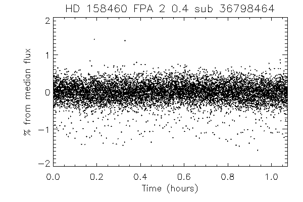
Relative stability of a bright star observed in subarray mode over a one hour time period.
3.4 Pixel Phase Correction
The flux density of a source measured using aperture photometry is a function of the location of the source centroid in a given pixel (the phase of the centroid with respect to pixel center). This variation is a combination of the detector undersampling with intra-pixel gain variations. Point source photometry should be corrected for this variation. The photometric variation is up to 8% at 3.6 μm and 4% at 4.5 μm where sources are fainter at the pixel corners. The S19.1 correction for this "pixel-phase" effect can be found here. The correction for the S19.2 data is folded into the correction for the array location-dependent corrections and can be found here.
3.5 Array Location-Dependent Photometric Correction
Based on our analysis of observations of IRAC calibration stars, the location-dependent photometric correction has changed from the cold IRAC correction. After the final array setpoint determination, a standard star (BD+67 1044) was observed over a densely spaced grid on each array and the position dependency of the photometry mapped. As with the cryogenic location-dependent correction, the variation is reasonably fit by a 2nd order polynomial in array coordinates (x, y).
For well-dithered data, the photometric variation should average out. Observations of sources towards the center of the array will also have minimal corrections.
For the S19.1 and S19.2 processings, correction images for the
location-dependent photometric correction can be downloaded
here
for channel 1 and channel 2. Be sure to use the right
processing version. If in doubt, please check the FITS header
keyword "CREATOR" for the correct processing version. Photometry
of blue sources (sources with SEDs falling with increasing wavelength)
should be multiplied by the value of correction image at the
centroid location of the source. For the S19.2 processing, the
location-dependent photometric corrections can also be applied using
the same routine that corrects for "pixel-phase" which can be found
here.
Note that this correction can be turned off (and it should
be off for sources with SEDs that are rising with wavelength).
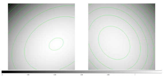
From the Warm SOM Figure 6.13: Photometric correction images at 3.6 microns (left) and 4.5 microns (right). The contours start at 0.95 for 3.6 microns and 0.94 for 4.5 microns and increment by 0.01. The correction images are normalized to the average response of the array.
4. Optical Properties of the Arrays
The optical properties of the telescope and instrument have not changed measurably since the cryogenic mission. The array locations and orientations are the same to within 0.1" in position and 0.1 degrees in rotation. Measurements of the array distortion also indicate no significant changes from the cryogenic mission to within measurement uncertainties ranging from 0.1 pixels in the array centers up to ~ 0.5 pixels in the array corners. The S19.2 processing contains an improved distortion solution using a 5th order polynomial representation which has a maximum uncertainty of 30 mas at the array edges. The S19.1 solution has residuals of 125 mas. Focus measurements also indicate that the focus has remained close to the cryogenic mission value.
5. IRAC Dark Frames
Since IRAC does not use a photon shutter for a dark measurement, a pre-selected region of low zodiacal background in the north ecliptic cap is observed to create a "skydark." During each campaign, a library of skydarks of all frametimes is observed, reduced, and turned into skyframes with the pipeline. In the cryogenic mission, laboratory measurements of the bias (obtained with zero illumination) existed, and were applied as "labdarks", prior to skydark subtraction. This labdark also corrected for bias variations that depended on the detector read history (known as the "first-frame effect"). The skydark then corrected for any additional temporal variation in the bias pattern.
However, no such laboratory measurements exist for the warm instrument. As a result, there is currently no correction for the first-frame effect, and so some floating bias level is seen in the BCDs. For the warm mission, skydark suites are taken, reduced, and used in the same manner as in the cryogenic mission. Overall, a higher bias level is seen in the skydarks relative to cryo. In addition, clusters of bad pixels at 4.5 microns result in a series of artifacts (notably column pulldown) being present in every frame. Since they are in every frame taken, they are mostly removed during the sky-subtraction stage in the pipeline. Median counts of the bias frames have increased significantly from ~ 30 DN/s in cryogenic mission to ~ 100 DN/s in warm mission in channel 1, and from ~ 3 DN/s in cryogenic mission to ~ 12 DN/s in warm mission in channel 2.
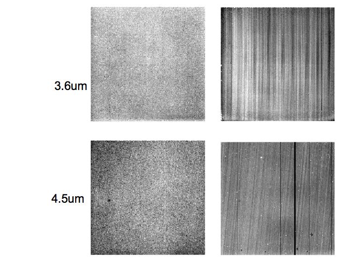
The above figure shows the IRAC 12 second skydark ensembles created in cryogenic mission (left) and during the warm mission characterization period (right). The column pulldown artifact is apparent in five columns of the 4.5 micron channel in the warm mission darks. Its strength is the same percentage of the background for all the frame times. The increased striping is a result of the more significant bias and not having a labdark subtracted.
6. IRAC Flat Fields
The pixel-to-pixel gain variations (commonly called the flatfield) were remeasured during IRAC Warm Instrument Characterization (IWIC) and again every two weeks during the regular warm mission. These measurements were made as during the cryogenic mission, using highly-dithered imaging of the brightest parts of the zodiacal cloud.
Overall, the flatfield has remained substantially unchanged relative to the cryogenic mission. There are, however, small gradients and other changes at the 1% - 3% level, so the two are not interchangeable. Similarly, the normalization of the flats has changed slightly, so for self-consistency the current flux calibration factors only apply to data processed with the new flats.
Data taken during IWIC and PC-1 through PC-4 are flattened using calibration data obtained during IWIC. The accuracy of the flat is 0.7% (1 sigma) at 3.6 microns and 0.3% at 4.5 microns. Data taken with the temperature floating (between August and September 2009) may have slightly degraded performance. However, given the very small differences in the flatfield between 15 K and 30 K, it is likely that the flatfield is still accurate to better than 1%. Data obtained on September 18, 2009 and later are flattened with data taken during the first three years of the warm mission. The accuracy of this flat is 0.17% (1 sigma) at 3.6 microns and 0.09% at 4.5 microns. As of S19.2, we have frozen the flatfield calibration and we will use subsequent flatfield observations to only monitor potential variations in the flat.
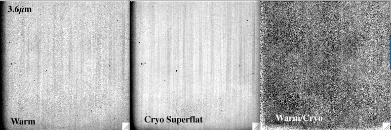
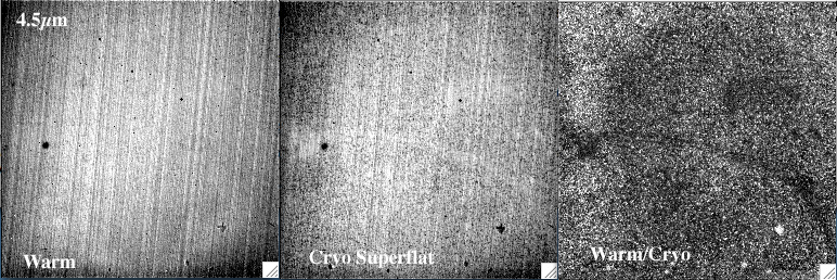 A comparison between the flats derived during IWIC and the cryogenic flats. Large-scale variations at the level of a few percent are seen.
The final warm skyflats are available in a tar file:
Warm IRAC Sky
flats.
7. IRAC Linearity
The IRAC detectors have a non-linear response - the conversion from detected flux to data numbers is not a simple constant. In the cryogenic mission, this non-linearity was corrected based on ground calibration of the instrument using special test equipment, and was confirmed in-flight through numerous observations.
During IWIC, it was found that the non-linearity and well-depth varied as both a function of applied voltage on the arrays and the array temperature. Both of these have been changed as a result of warm operations. Unfortunately, it is extraordinarily difficult to recalibrate the linearization in-flight with the accuracy of the ground-based cryogenic linearization.
For S19.1, the linearity calibration was derived using a combination of staring observations of bright galactic nebulae, and from the photometry of sources observed by the SERVS Exploration Science program, versus the same sources observed by the SWIRE Legacy science program during cryogenic operations. The final linearity solution applied in the S19.2 processing includes additional adjustments incorporating the constancy of the PSF as a function of well depth. The new linearity solution should be accurate at alevel of better than 0.5% up to above 90% full well. The cryogenic calibration is still used for the period prior to September 18, 2009 while the new warm linearization is used for all data taken afterwards.
IWIC results indicate that the non-linearity at warm temperatures is more severe than at 15 K. Using the cryogenic calibration provides at least a partial correction. Note that the flux calibration is based on standard stars which are usually near 1/3-1/2 full well. Targets that are near this well-depth will always have correct fluxes. Warm data linearized with the cryogenic calibration in channel 1 will have a systematic error of roughly 2%-3%, such that brighter objects (those approaching the saturation limit near 30,000 DN) are systematically too faint. The effect is much smaller in channel 2, and is believed to be approximately 1%. In addition to bright objects being too faint, faint objects may appear slightly brighter than they actually are, although this effect will be at the 1% level or less.
The other change in the warm linearization is that the well-depth which is defined by the point at which the pixel DN peaks is now roughly 30,000 DN in both channels, whereas it was closer to 44,000 DN in the cryogenic mission. For data processed with the cryogenic calibration, the saturation flag should be considered unreliable. Users should examine the raw data numbers for sources that are suspected of being near saturation.
8. Persistent Images
Both IRAC channels have residual images of a source after it has been moved off a pixel. When a pixel is illuminated, a small fraction of the photoelectrons is trapped. The traps have characteristic decay rates, and can release a hole or electron that accumulates on the integrating node long after the illumination has ceased. The warm mission short-term residual images are different in character than the cryogenic residuals (for details on the cryogenic residual images, see Section 7.2.8 in the IRAC Instrument Handbook), as the behavior of the trap populations is a function of the impurity type and temperature. Typically for channel 1, warm residuals are <0.01% of the fluence of the source after 60 seconds. The residual image never exceeds 1% of the illuminating source for integrations beginning immediately after the illumination ends. Usually the residual will be orders of magnitude smaller, but the residual image of a star can persist as a false point source for up to several hours for the most saturating sources followed by low background deep observations. Channel 2 residual images decay much more rapidly than those in channel 1, lasting at most 10 minutes for the brightest sources.
For reference, the first figure below shows the residual decay for a strongly saturating first magnitude source observed in a 12 second integration time in channel 1. The data residuals are measured using aperture photometry of subsequent frames and the residuals are averaged over time. In this extreme example, the residual persists above the noise in the background for more than five hours after the residual is produced.
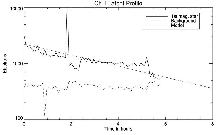
Residual image brightness decay as a function of time interval since exposure to a first magnitude source at 3.6 μm. The residual is compared to three times the noise in the sky background as measured in an equivalent aperture. The fitted exponential decay function is plotted as the dot-dashed line. These curves have been smoothed to mitigate flux jumps due to sources at the position of the original source in subsequent images.
An example of the residual images for channel 1 is displayed in Figure 6.12 which displays the residuals produced by 3rd and 4th magnitude stars observed in a 12 second integration. In addition to the compact residuals, there are streaks that can be produced when bright sources cross the array during slews between AORs.
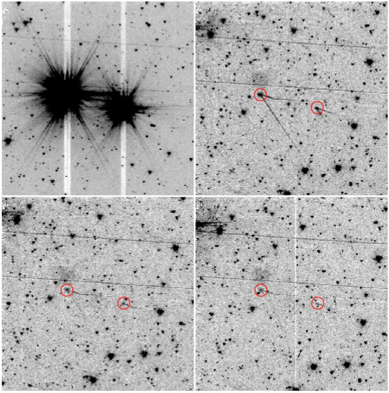
(From the Warm SOM, Figure 6.12): Illustration of residual images in warm data. 3rd and 4th K-magnitude stars were observed in a single 12 second frame (upper left panel). The upper right, lower left and lower right panels show the decay in the residual in 12 second frames taken 60, 120 and 180 seconds after the bright sources were observed. The positions of the bright sources on the array are identified by red annuli in subsequent frames. The linear features connecting to the bright residuals are from slews, produced as those bright sources move on and off the array. The dark patch above the 3rd K-magnitude star residual (leftmost residual) is a diffuse residual from a previous observation and the linear features crossing the entire array are slew residuals from bright sources crossing the array during earlier observations.
9. Muxbleed
The muxbleed artifact no longer occurs at the final warm array temperature. The correction has been turned off in the pipeline.
10. Column Pulldown
Column pulldown has been identified in the warm data, but is more severe; additionally there are several columns in channel 2 that are now permanently pulled down due to hot pixels. The level of the pulldown above and below the triggering source is different, and the pulldown decreases with distance from the trigger along the column. Third order polynomial and exponential fits to the data appear to work well, although they are complicated when dealing with complex backgrounds. The triggering threshold in any given frametime is considerably smaller than in the cryogenic mission.
11. Saturation
The saturation level has changed slightly in the warm mission as a result of changes in well-depth and sensitivity. Additionally, users should be aware that for certain frametime/Fowler-number combinations the saturation values (in DN) differ significantly from the norm, and that the saturation value varies across the array. This effect is greatest for the shortest frametimes. In general, the highest saturation levels are near the bottom left corner (pixel 1,1). Note, however, that deliberately placing a specific target near a pixel corner rather than a pixel center is a much more effective strategy for coping with saturation than manipulating overall placement on the array. Using a pixel corner will increase the saturation level in the table below by factors of roughly 3-4. The table below gives the array-averaged saturation limits for a source centered on a pixel in each channel as a function of frametime.
| Frame Time (sec) |
3.6um sat (mJy) |
4.5um sat (mJy) |
|---|
| 100 |
2.8 |
3.5 |
| 30 |
10 |
12 |
| 12 |
25 |
30 |
| 6 |
50 |
60 |
| 2 |
160 |
200 |
| 0.6 |
500-700 |
600-900 |
| 0.4 |
900-1400 |
1000-1700 |
| 2 subarray |
150 |
180 |
| 0.4 subarray |
700 |
900 |
| 0.1 subarray |
3000 |
3700 |
| 0.02 subarray |
20000-26000 |
28000-35000 |
A more detailed discussion may be found here.
12. ABADDATA - Extra Pixel in Science Image
An occasional problem is observed during the warm mission wherein an extra byte appears in the science packet (image data). As a result, all pixels after this byte are shifted by one pixel. Such images are identified by having the ABADDATA header keyword set in the raw data (BADTRIG in the BCD images); the images themselves usually become stripy as a result of the mismatch between the science and calibration data. The SSC pipeline corrects this by locating the first pixel in the image with a value of exactly 0, and then shifting all later pixels. This correction may fail if there are multiple zero-level pixels in the image.
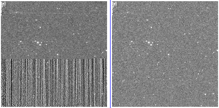
Illustration of processed BCD with ABADDATA (left) and after correction (right).
13. Bad Pixels
The location of the quasi-static bad pixels changed relative to the cryogenic mission. Quasi-static bad pixel masks for both the cryogenic and warm missions can be downloaded here.
Bad pixels in channel 1 (left) and channel 2 (right), in BCD orientation.
* Copyright Society of Photo-Optical Instrumentation Engineers. One print or electronic copy may be made for personal use only. Systematic reproduction and distribution, duplication of any material in this paper for a fee or for commercial purposes, or modification of the content of the paper are prohibited.
|