Background subtraction is performed by the same MedFilter module that is used in the Mosaic pipeline. The program computes an asymmetrically skewed median for each pixel in the input image using a rectangular window of Window X by Window Y size. It is achieved by omitting Outliers / Window highest pixels from each median window. If Outliers / Window is set to 0 the program calculates the regular median. There is also the option to use the faster Sbkg background fitting method, like that used by SExtractor.
Postage Stamp Image Creation
The Crop Stack module cuts out postage stamp images from the input images around each point source from the input Point Source List. If a single input image name is specified, then the postage stamps are cut out from that image. If a list of images is specified, then the postage stamp images are cut out from each image listed therein. The position of the point sources in the input list can be given in sky coordinates or in pixel coordinates. In the latter case, a Fiducial Image Frame table is required (see §5.6.4).
PRF Estimation
The PRF Estimate module computes a PRF image(s) (see §8.7) based on the input images of an isolated point source, not necessarily the same source, just a single source. An attempt is made to automate the process of weeding out bad images from the process of PRF estimation using several outlier rejection mechanisms and using data fitting to determine input point sources flux and positions. However, it is up to the users to verify that these efforts were ultimately successful, especially if they suspect that the PRF produced by the program has some problems.
The software has an option of creating either a single PRF image for the whole array or a set of PRF images for the different sectors of the detector array. The mapping of the detector array into sectors is specified in a file called a PRF map. The assignment of postage stamps to different parts of the array is performed in the Split By Array Position module. After that, the PRF Estimate module runs consecutively on each partial list and a PRF image is created and saved for each detector array sector.
There are four steps in creating a PRF: NaN replacement, exact point source position and flux estimation, outlier rejection, and coaddition.
NaN Replacement: The program replaces each NaN in the input image with the median of a number of the neighboring pixels.
Extract Point Source Flux and Position Estimation: For both outlier rejection and coaddition, each input postage stamp image is shifted to the common grid, in which the peak of the point source position coincides with the center of the central pixel. By default the position of the point sources in the input images are computed as flux weighted centroids. Each postage stamp image is normalized by its flux. The flux can be given in the input point source list. If it is, then the column name of the appropriate column should be 'flux' or can be specified in the PRF Estimate module by the parameter Flux Column Name. If the flux is not given in the input table, then it is found by summing all the pixel values in the input image.
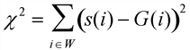
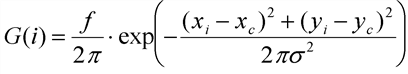
The flux and the exact position of the point source in each Postage Stamp image are estimated by fitting the data with a Gaussian. The following quantity is minimized:
Equation 7.1
with respect to the flux f, width σ, and position (xc,yc) of the point source in the Postage Stamp image. Here s(i) is the pixel value of the input image for pixel i, W is the area in center of the image. The size of the area is specified with the PRF Estimate module parameters Fit X, Fit_Y both defaulting to 5 pixels. Simulated annealing method is used to minimize χ2.
Outlier Rejection: Two kinds of outlier rejection are performed. The first kind is when the whole image is rejected based on some criteria. The second kind is when only some pixels in an image are detected as outliers and then replaced with some combination of the neighboring good pixels.
Image rejection is done based on several different criteria. Two of the criteria are: having too many NaN's in the input image, or having a NaN pixel in the central box. Two criteria are based on the results of the Gaussian point source fitting (see above), specifically using the values of σ and χ2 for each image. The third criterion is the number of outlier pixels detected in the image. The fourth criterion is having an outlier pixel in the central box of the image.
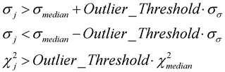
After Gaussian fitting is completed for all input images the sets of σ and χ2 are analyzed. Image j is declared an outlier, if any of the three conditions below are met:
Equation 7.2
Here the subscript median indicates the median value of the quantity and the subscript σ indicates its standard deviation.
Next step is detecting and rejecting pixels outliers. For the outlier rejection step, no resampling is performed. The input images are shifted to the common grid using the bicubic interpolation. The shifted images are stacked up and outliers are found. The parameter Outlier Threshold specifies the number of trimmed sigmas below and above the trimmed mean to be used to determine the outliers. If a particular image has too many outliers it is completely rejected from further processing. “Too many” is determined by two parameters: if the fraction of the outliers in an input image is greater than Max Ratio Outliers and the total number of the outliers is greater than Max Number Outliers then the image is rejected. An image is also rejected if the outlier pixel is found in the center of the image, the center being defined the same way as it is for the NaN pixels: it is specified with the input parameters (Center Box X, Center Box Y), both defaulting to 7. If an image has a number of outliers but is not rejected, then the values of the outlier pixels is replaced with the median of the neighboring pixel values in exactly the same way the NaN's are replaced in the input images. There is an additional step of re-projection of the shifted images back on the input images, since the outlier detection is performed on the shifted images. A pixel in an outlier image is considered an outlier if the fractional area overlap of the pixel with the outlier pixels from the shifted image is greater than Min Outlier Overlap.
Resampling and Combining: For coadding, the input images are resampled and shifted to the common grid using the bicubic interpolation. The ratio of the pixel sizes to the sampling distance is given by the parameters PRF Resample X Factor and PRF Resample Y Factor. The resampled and shifted images are stacked up and a simple mean and standard deviation are found for each pixel position.
Output
If the Split By Array Position module is included, then the names of the output files are read from the PRF map, in which case the parameters PRF filename and PRF Sigma Filename are ignored if given in the Initial Setup. Otherwise, these parameters can be used to specify the names of the output images with the default names PRF.fits and PRFSigma.fits. A coverage map is output if PRF Coverage Filename is specified in the Initial Settings.