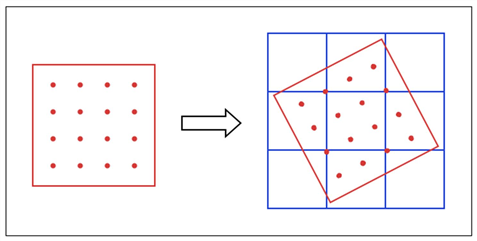
The Mosaic Interpolate module (see e.g. �5.6.8) performs a projection of input images onto the Fiducial Image Frame (FIF; see e.g. �5.6.4) and an interpolation of the input pixel values to the output array of pixels of the user-defined pixel size. It corrects for the optical distortion in the input images. The process is intended to, but not restricted to, accept images measuring surface brightness and to yield images in the same units.
The FIF defines the sky position, orientation, and the size of the mosaic. The final mosaic pixel size is set in the Initial Setup module with the options Mosaic Pixel Size X(Y) or Mosaic Pixel Ratio X(Y). On the command line, it is set with the namelist options MOSAIC_PIXEL_SIZE_X(Y) or MOSAIC_PIXEL_RATIO_X(Y). See �5.6.1 for more information.
Four interpolation schemes are implemented: Default, Drizzle, Grid and Cubic. The first two schemes are based on area overlap, but they differ in the way the projection is done. The third scheme is a rough approximation of area overlap. The fourth scheme is the bicubic interpolation, which is a common technique in image processing.
Whatever interpolation scheme is used for the input images, the uncertainty images are interpolated in an identical fashion. A coverage map is created for each interpolated image. It reflects the presence of any input bad pixels or pixels on the edge of the input image.
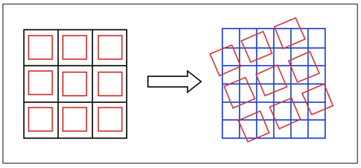
In general, a projection onto the reference frame of an input image with optical distortions will not be a simple rectangle. Each interpolated image occupies a part of the FIF and is, in general, of different size with different offsets from the origin of the FIF. The offsets of the interpolated images in x- and y- directions relative to the FIF, and their sizes (in integral numbers of pixels) are given in the file interpolated_images.txt.tbl, and also written in the headers of the interpolated images in the keywords MINTOFFX and MINTOFFY.
For maximum speed of operation, a special set of routines have been developed that allow direct plane-to-plane coordinate transformations that bypass computing the sky coordinates. For details, see the document �Fast Direct Plane-to-Plane Coordinate Transformations� (Makovoz 2004, PASP, 116, 971; http://www.journals.uchicago.edu/cgi-bin/resolve?PASP204097).
8.4.2 Default: Pixel Overlap Integration
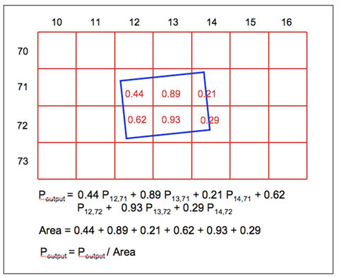
The value Oj of an output interpolated pixel j is equal to the weighted average of the input pixels Ii overlapping the output pixel. It is weighted with the relative overlap areas as follows (Eq. 1):
where
Equation 8.11
Here ajiis the area of the overlap of output pixel j with input pixel i.
For this scheme (see Figure 8.16), each output pixel is projected onto the input image frame and the flux from all the input pixels overlapping the output pixels is integrated and then normalized by the output pixel area to yield the result in the units of surface brightness.
If the Fine Res (FINERES on the command line) keyword is specified in the Mosaic Interpolate module, an additional bi-linear interpolation of the input pixels is performed before projecting onto the output grid. A grid of fineres pixels with the size defined as Input_Pixel_Size/Fine Res is introduced. In Figure 8.17 the input pixels are shown in thick black lines, the intermediate fineres pixels are shown in thin black lines. The value of a fineres pixel is a linear interpolation of the four closest input pixels, with the interpolation coefficients being the relative overlap area of the pixel, with the same size as the original input pixels, and centered around the fineres pixel. i.e. the value FP of shaded fineres pixel in Figure 8.17 is equal to:
Equation 8.12
where IPi is the value of input pixel i, and Ai is the overlap area of pixel i with the pixel (blue fat lines) centered around the shaded pixel, with the same size as the input pixels. The output pixels are then computed using the pixel overlap interpolation scheme with the fineres pixels used as the input pixels.
Figure 8.16: This figure shows the calculation of the weighted sum of the input image pixels (red, regular grid) overlapping the interpolated output image pixel (blue, thick line).
Figure 8.17: Fine Res = 4. The coordinates of the shaded pixel are j = 2, k = 2.
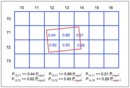
8.4.3 Drizzle: Pixel Overlap Distribution
The output pixels values are computed using Eq.1, just like in the previous scheme. The difference is that for this scheme (see Figure 8.18) the input pixels are projected onto the output frame. The flux of an input pixel gets distributed among the output pixels it overlaps.
Each input pixel is shrunk by the factor Drizzle Factor (DRIZ_FAC in command-line namelists). The values of the shrunken pixels are equal to the values of the original pixels. The shrunken pixels are projected onto the output image frame. This would be extremely hard to implement using scheme one, since then the overlap with the non-contiguous array of pixels would have to be computed (see Figure 8.19). On the other hand scheme one has been shown to be faster by ~25% than scheme two in the case of no drizzle, Drizzle Factor = 1.
Note: When using the Drizzle option, several of the mosaicking steps are run twice. Firstly, a linear interpolation is carried out so MOPEX can run the outlier rejection scheme. Once the outlier rejection masks (RMasks) have been created, MOPEX returns to the Mosaic Interpolate module and re-runs the interpolation with the Drizzle algorithm, masking out any pixels flagged in the RMasks. When using this option, do not include the Mosaic Reinterpolate module in the processing flow.
Figure 8.18: This figure shows the calculation of the weighted contributions of the input image pixel (red, thick line) to the overlapping interpolated output image pixels (blue, regular grid). The area of each output pixel in the output coordinate system is constant.
Figure 8.19: Input pixels are shown in black. The drizzle pixels, shown in red, are projected onto the output array of pixels shown in blue.
8.4.4 Grid Distribution
As a fast alternative of the area overlap method the grid interpolation is implemented. Each input pixel is filled with Grid Ratio (GRID_RATIO) squared grid points (see Figure 8.20). Each grid point is assigned the value of the pixel it belongs to. Each grid point is projected onto the output frame and the flux associated with the grid point is added to the output image pixel into which the grid point was projected. The value Oj of an output interpolated pixel j is equal to the weighted average of the input pixels Ii
where
Equation 8.13
where nji is the number of the grid points projected into the output pixel j from the input pixel i. The parameter Grid Ratio specifies the number of grid points in one direction in an input pixel. In other words there are Grid Ratio squared grid points per input pixel. If Grid Ratio = 1 and the input to output pixel size ratio PR = 1, the method is equivalent to the nearest-neighbor interpolation. In the limit of infinite Grid Ratio the method approaches the area overlap interpolation. The main purpose of this scheme is to create first-look mosaic images fast, the gain in speed being up to 10 times as fast as scheme one. The price you pay is the fidelity of the interpolated images. Do not use these images for science.
Figure 8.20: Input pixel (red) is filled with a grid of points. When the input pixel is projected onto the output array (blue) each point contributes an equal share of the input pixel value to the output pixel it is in.
8.4.5 Cubic: Bicubic Interpolation
For the bicubic interpolation the value O(j) of the output pixel j is computed as a linear combination of the input pixel values
Equation 8.14
at the 16 positions i closest to j. The coefficients C(j,i) depend on the distance between the points:
Equation 8.15
The coefficients aklare derived by imposing the following constraints h(0) = 1; h(1)=h(2) = 0;h'(1) and h'(2) are continuous. These constraints yield seven equations for eight unknown coefficients. By allowing a31= α the tunable parameter the system can be solved and the results are shown in the Table below. The parameter α is set in the interpolation module, with the default value equal to -0.5.
 where
where 
 where
where