The Extract module performs spectral extraction within a user-specified window. The resulting one-dimensional spectrum is in units of electrons per second and will be used as input to the flux conversion modules, Point Source Tune and Extended Source Tune.
Exract can be used in three separate modes: Regular, Optimal, and Extended. Each is offered in its own Generic Template, but the user can switch between them by changing the appropriate settings.
INPUTS
Optimal or Regular Extract: This menu allows the choice between standard (point or extended source) or optimal extraction.
NaNs: SPICE can optionally interpolate over NaN pixels in the data. Choose Replace NaNs to perform the interpolation, otherwise choose Do not replace NaNs. NaNs can be present in IRS BCDs when there is no good data available for that pixel.
Uncertainty (Constant or File; Optimal Only): During optimal extraction, each pixel in the aperture is weighted by the Signal-to-Noise squared. By default, the input uncertainty file (supplied in Initialize Parameters and Files module) are used for as the Noise. To keep the default, retain the UseFile choice in the pulldown menu. Alternately, by choosing SetConstant, the user can enter a constant uncertainty value (in electrons per second) giving a purely profile-weighted extraction. This option is appropriate for sources that are fainter than the background and where background noise dominates, or where the input file has poor uncertainty estimates. The output uncertainties will reflect whatever constant is entered rather than the true uncertainty.
Constant Uncertainty: The user-specified constant uncertainty for profile-weighted extraction. This field is only active if SetConstant is chosen for the type of uncertainty in optimal extraction.
Set Fatal Bit Pattern: The BMask defines the status of each pixel using bitwise encoding. Pixels in which fatal bits are set will be excluded from the extraction. The fatal bits can be defined by the user by choosing Select Bits and using the checkbox menu to the right; otherwise, retain the Default. See §1.6 for a list of bit definitions.
PS or ExtSrc: Choose Point Source – Default, Point Source - Manual, or Extended Source - Full (28 pixels) to define the width of the low-resolution extraction aperture. In the high-resolution slits, this module extracts a 1D spectrum from the full slit. In the low-resolution slits, the spectrum is extracted along the Ridge location in accordance with the wavelength-dependent Point Spread Function (PSF) and the spectral trace. The Extract module can employ a window with a different width, but the width will still scale with wavelength. Alternately, an extraction window with constant width may be used by specifying λ = 0 for the reference wavelength.
Note: The only properly calibrated, non-point-source width extraction is the extended source 28 pixel width. Flux conversion factors are based on standard width extractions, as defined by the psf_fov.tbl files. Non-standard extractions will still be converted from electrons per second to Janskys, but the conversion factors will be incorrect.
Note: A very wide manual window can potentially cause the extraction of pixels between the orders, or even in a different order. Inter-order pixels will be masked if bit #8 is set as fatal and Spitzer BMasks are used. To check the fatal bits, use the Select Bits option in Set Fatal Bit Pattern (see above). Be sure to visually inspect the extraction window overlay to avoid including pixels from a different order.
Width (pixels): The width of the extraction aperture (at the reference wavelength) in pixels. This field is only active for user input if the Manual point source extraction option is chosen.
Wavelength (um): The reference wavelength for the extraction aperture (set to zero for a constant, non-expanding width).
OUTPUTS
Spectrum (*.extract.tbl): The output of the module is the one-dimensional extracted spectrum, in units of electrons per second. The spectrum is written to the table in the output directory and displayed in the plot window. An ASCII version of the file is seen by clicking the View button.
Rectified products (Optimal only): If optimal extraction is used, additional products are output. They are the rectified version of the 2D spectrum, uncertainty, BMask, and spatial offset files. The rectified versions are named: *.rectified_flux.fits, *.rectified_unc.fits, *.rectified_bmask.fits, *.rectified_offset.fits.
DISCUSSION
Settings: The Extract module can be used in three separate modes. Usually the choice of mode will be made at the beginning when choosing a Generic Template for the flow. It may occasionally be convenient to switch modes mid-stream. To do so, each mode requires setting the parameters to appropriate values:
Regular: Set Optimal or Regular Extract to Regular; set PS or ExtSrc to one of the point source options. Other parameters may be modified if necessary. Make sure the Point Source Tune module is enabled.
Optimal: Set Optimal or Regular Extract to Optimal; choose whether to modify the uncertainty weighting (see above); set PS or ExtSrc to one of the point source options. Other parameters may be modified if necessary. Make sure the Point Source Tune module is enabled.
Extended: Set Optimal or Regular Extract to Regular; set PS or ExtSrc to the Extended Source option. Other parameters may be modified if necessary. Make sure the Extended Source Tune module is enabled.
Only one tuning module should be enabled. To disable a module, use the "X" button in the upper-right corner of the module box. To enable a module, click the "Enable" button.
2.5.1 Standard Spectrum Extraction
The Extract module takes the dispersed BCD image and extracts the 1-D spectrum along the trace defined by ridge.tbl. The module takes as input the data array, bcd.fits and the associated uncertainty plane and pixel status bitmask; it also takes the output of Ridge, which defines where the extraction is to be performed.
In the high-resolution slits, this module extracts a 1D spectrum from the full slit. In the low-resolution slits, the spectrum is extracted along the Ridge location in accordance with the wavelength-dependent Point Spread Function (PSF) and the spectral trace. The width of the extraction is defined in the psf_fov.tbl file, which gives the width to employ at a fiducial wavelength for each order. The width of the extraction scales with wavelength in all low resolution slits, under the assumption that the spectrum is diffraction limited. However, the width does not scale between sub-slits. Rather, the extraction width has been empirically determined for each subslit, and wavelength scaling is performed within each individually. The exception to the wavelength dependent window width in low resolution is the case of observations taken in the "Both" fields of view; that is Long-Low-Both or Short-Low-Both. In that case, the default is to perform a full slit extraction. Also, the user may demand a non-scaling width by setting the reference wavelength to 0 when selecting a manual extraction width.
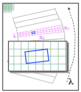
The source spectrum incident on the array is not rectilinear in either the spectral or cross-dispersed direction. As a result, the Extract module does not extract whole pixels, but rather subdivides the array into a network of polygon-shaped sampling elements referred to as “pseudo-pixels” (see Figure 2.5.1), which lie within the “pseudo-rectangle” that defines each wavelength in each order (specified in the wavsamp.tbl file). Pseudo-pixels do not necessarily overlap the rectangular pixel grid. These elements allow Nyquist sampling of spectra in the dispersion direction. Extraction is performed by calculating the signal that falls within the boundary of the “pseudo-rectangles” which lie within the extraction window. Light is assumed to be evenly distributed within a pixel for purposes of calculating fractional contribution.
Figure 2.5.1: (Left) A pseudorectangle is divided into pseudopixels. The pixels form the FITS image for a rectangular grid, as illustrated in the upper left corner. (Right) A pseudopixel is shown against the pixels of the original FITS image. The pseudo pixel contains partial FITS pixels, so each partial pixel must be carefully accounted for to perform the extraction.
The input pixel-status bitmask is used to define "fatal" bit-flags to identify pixels that will be excluded from the average of the pseudo-rectangle. The extraction depends on the processing version and the module:
· For S18.7, for SL, LL and LH data, the extraction is the sum of signal in the non-flagged pixels at each wavelength divided by the height (measured along the spectrum in pixels) of the extraction window, as set by the wavsamp wavelength calibration file. For SH, the extraction is the sum of signal in the non-flagged pixels at each wavelength divided by the number of (fractional) pixels;
· For S18, only LH spectra were divided by the wavsamp height;
· For previous processing versions, no modules had spectra divided by wavsamp height – all were simply the sum of the signal in the non-flagged pixels at each wavelength, divided by the number of (fractional) pixels.
Note that unflagged bad-pixels (NaN or zero DN) are not included in the calculation of the value of the extracted flux. Alternately, the NaNs may be interpolated over and included, by selecting that option in the module input switches.
The uncertainty defined in the input uncertainty plane is propagated into the extracted output spectrum. The output spectrum table includes the order, wavelength, flux (in electrons per second), propagated error, and cumulative pixel status for each wavelength. The cumulative pixel flag is a bit-wise OR of the flags of contributing pixels.
2.5.2 Extended Source Extraction
In addition to the standard point source extraction, the Extract module in SPICE offers the users the ability to estimate the surface flux for particular extended sources.
The calibration assumes that the source is infinitely large in the sky, and that at each wavelength the source is uniform. Starting from the extracted spectra, two corrections are applied: one for light losses due to the extraction aperture, and another for light coming in and out of the slit due to diffraction. We describe each in turn here. A more formal discussion is provided in the IRS Instrument Handbook.
In the calibration of point sources, SPICE uses an expanding aperture for the low-resolution modules, and the full slit for the high-resolution ones. For extended sources, a straight-edged 28-pixel extraction aperture is used for the low-resolution modules (which allow us to ignore the noisy edge pixels). The full slit is used for the high-resolution modules. Appropriate calibration coefficients (“fluxcon values”; see §1.5) are applied to the low-res modules to account for the large extraction window and are provided in b[0,2]_aploss_fluxcon.tbl. These fluxcon values assume a point source centered on the slit. For a point source, the difference in e-/s between the point and extended source apertures is at most ~10%. When the user clicks the extended source button, the fluxcon table for the large aperture is applied to convert from e-/s to Jy. Note that no such correction is necessary for the high-resolution modules -- they will have the same fluxcon table for the point source and extended source calibrations.
The slit losses are a function of wavelength. For point sources, the flux lost due to the PSF wings outside the slit is added back by comparing the signal to a model. For a source that is uniform in flux at a given wavelength and infinitely large, the light lost from the slit is exactly matched by the light gained by the slit. Because the point source calibration adds the flux from the wings outside the slit in order to derive the final calibration, this calibration must be "undone". To understand the wavelength dependent loss of light, the point spread function was simulated using a STinyTim model with the slit sizes quoted in the IRS Instrument Handbook. The slitloss correction was taken to be the ratio of the flux within the slit of a simulated PSF, to the total PSF flux. The slitloss corrections are given in (b[0,1,2,3]_slitloss_convert.tbl), which have the wavelength dependent factor by which the spectrum of the extended source should be multiplied.
To convert the resulting spectrum in Jy to a surface brightness, the user should divide it by the area of the aperture in the sky (or the area of the extraction window, if the default was not used):
Table 2.5.1: Slit dimensions for the IRS modules
Module name Slit Length Slit Width Solid angle
(arcsec) (arcsec) (arcsec^2)
----------- ----------- ---------- ------------
SL2 50.4 3.6 181.44
SL1 50.4 3.7 186.48
LL2 142.8 10.5 1499.40
LL1 142.8 10.7 1527.96
SH 4.7 11.3 53.11
LH 11.1 22.3 247.53
After this process, it is likely that the spectra from different modules will not match each other. Most extended astronomical sources have spatial and spectral structure that cannot be accounted for a-priori by any calibration set. It is recommended that the users compare their data to other photometric measurements (like MIPS-24 data) to achieve better calibration. Note that IRAC channels 3 and 4 need post-pipeline processing to be usable for extended emission (see the IRAC Instrument Handbook).
2.5.3 Optimal Extraction
In the Extract module, the user has the option to select profile-weighted and signal-to-noise weighted “Optimal” extraction. This option can be selected in the pulldown menu under the Extract module. The default is “Regular” unweighted extraction. The name of the output file is the same, regardless of which option is chosen. Optimally extracted spectra may be identified by the information in the table header.
The “Optimal” algorithm yields a minimal-noise, unbiased flux estimate in each wavelength bin (Horne, 1986), by weighting the extraction by the object profile and the signal-to-noise of each pixel. Specficially, the flux density (electrons per second) in a wavelength bin, F, is given by:
Equation 2.1
where Wi is the weight,
Equation 2.2
Fiis the flux, Pi is the stellar profile template, and σi is the uncertainty in the ith pixel.
This extraction is accomplished as follows by the Optimal Extract module. First, the dispersed image of the source is divided by the dispersed image of a standard stellar point source. At each wavelength, the flux of the standard template is normalized to unity, and the peak is shifted to the center of the extraction window. Next, each pixel in the aperture is weighted by the Signal/Noise squared, and the weighted average flux is computed.
By default, the input uncertainty file (supplied in the SPICE Initialize Parameters and Files module) and a standard point-source profile are used to compute the weights and output uncertainties. Alternatively, the user can enter a constant uncertainty value (in electrons per second) giving a purely profile-weighted extraction. This option is appropriate for sources that are fainter than the background and where background noise dominates, or if the uncertainty file is noisy. The output uncertainties will reflect whatever constant is entered rather than the true uncertainty.
To facilitate alignment of the source to the standard profile, optimal extraction is performed in rectified space. The curved BCD image is straightened using the wavsamp.tbl calibration file. Because the Spitzer PSF is under-sampled by IRS pixels and the spectral trace does not follow columns exactly, diagonal stripes are visible in rectified spectral images. Each order is rebinned during rectification to 1001 pixels in the spatial direction to increase the accuracy of the rectification and avoid pixelization error at the edges of the aperture. Unweighted extractions in rectified space match regular extraction to better than 1%.
Rectified flux, uncertainty, and BMask products are written out, allowing the user to inspect the spatial profile of the source or construct custom profile templates. These files are by default given names ending with .rectified_[flux,bmask,unc].fits. The wavelength and spatial scale of the rectified image is described by the wavsamp.tbl file for the appropriate order. In that table, each row describes the extraction pseudo-rectangle' for each extracted wavelength. In the rectified image, the rows in each order correspond to rows in the wavsamp.tbl for that order, and the row wavelength is given explicitly in the table. The orientation of each order in the rectified image is the same as in the BCD image (e.g. for SL-1 the blue end is at the top of the dispersed image and the red end is at the bottom). The spatial scale of each row is slightly complicated to calculate. It is given by the length of the pseudo rectangle (described by X0, Y0, X1, Y1, X2, Y2, X3, Y3), multiplied by the plate scale of the module (e.g. 1.8 arcsec/pix for SL) and then divided by 1001 (the number of columns in the rectified order). The rectified_offsets.fits files give the spatial offset for each pixel in the rectified image.
The rectified stellar templates used for point-source profiles are provided in the SPICE cal/ directory, one for each channel, order, and standard nod position (including nod 1, nod 2, and slit center) with filenames like:
b[channel]_rectempl_[order][nod].fits
These were constructed with Spitzer IRS observations of the flux calibration standards HR 7341 (1 Jy at 12 microns; SL and LL) and Xi Draconis (11 Jy at 12 microns; SH and LH). SPICE will automatically select the appropriate profile template for the channel and order using the BCD header FOVID keyword. The template closest to the selected ridge location will be used. Sources in the non-commanded order can be extracted using the “Orders” pulldown menu under the PROFILE module.
Optimal extraction provides greater improvement (over regular extraction) for low S/N data. Figure 2.5.2 shows the gain in optimal S/N vs. S/N in the regular extraction. Gains in S/N up to a factor of 2 have been achieved for sources with S/N ~ 3, corresponding to an effective quadrupling of the exposure time. There are diminishing returns for sources with S/N > 30. Comparable gains in S/N have been achieved by narrowing the extraction aperture to about 3 pixels and performing a regular extraction. However, the latter method requires custom flux calibration, and is still sub-optimal, in principle.
No special steps are required prior to optimal extraction; run Profile then Ridge, as you would before regular extraction. Note that optimal extraction is more sensitive to the Ridge location than regular extraction. For faint sources where the profile is noisy, the Ridge percentage can be refined manually until the best result is obtained. Optimal extraction may be performed in Batch mode by first selecting Optimal in the Type pulldown menu under the Extract tab. After optimal extraction, use the Point Source Tune module to create a properly calibrated spectrum. (For nonstandard apertures, custom flux calibrations may be necessary.)
Optimal extraction works best for point sources observed in IRS Staring mode, at the standard nod positions (33%, 66%) or at the center position (50%). For sources observed at non-standard locations along the slit, Optimal Extract will choose the closest stellar template, in terms of Ridge percentage. However, low-frequency sinusoidal wiggles may appear in optimally extracted spectra if there is a mismatch with the stellar template.
The user can create custom rectified stellar template (rectempl) by Optimal extraction of a bright star observed at the same Ridge percentage as the science target. The rectified 2D stellar spectrum is output as a standard Optimal extraction product.
Optimal extraction of extended sources has not been tested. If a standard point source profile is used, the center of the object will be weighted more than the outskirts. An extended source profile could be constructed and used, but it must incorporate pixelization effects, and must have an S/N greater than that of the spectrum to be extracted in order to achieve any gain. Do not use Extended Source flux calibration for optimally extracted spectra. The Extended Source Tune function assumes the science target uniformly fills the slit, whereas Optimal extraction assumes a point-source cross-dispersion profile.
Figure 2.5.2: Gain factor for Optimal extraction over Regular extraction as a function of Regular Signal/Noise for standard extraction apertures, derived from SL and LL observations. Diminishing gains are obtained for bright sources with S/N > 30. Maximal gains of > 2 are possible for faint sources with S/N < 5. The lowest S/N considered for Regular extraction is S/N = 1.5.