Stray or scattered light on the arrays can be produced by illuminating regions off the edges of the arrays. Stray light from outside the IRAC fields of view is scattered into the active region of the IRAC detectors in all four channels. The problem is significantly worse in channels 1 and 2 than in channels 3 and 4. Stray light has two implications for observers. First, patches of stray light can show up as spurious sources in the images. Second, background light, when scattered into the arrays, is manifest as additions to the flat-fields when they are derived from observations of the sky. The scattered light is an additive, not a multiplicative term, so this will result in incorrect photometry when the flat-field is divided into the data unless the scattered light is removed from the flat. Stars which fall into those regions which scatter light into the detectors produce distinctive patterns of scattered light on the array. We identified scattered light avoidance zones in each channel in which observers were told to avoid placing bright stars if their observations were sensitive to scattered light.
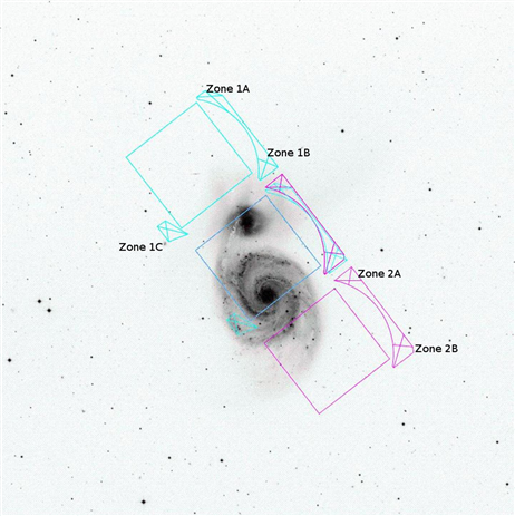
Figure 7.13: An image of the M51 system, showing an overlay of the IRAC fields of view, with the scattered light origin zones for channels 1 and 2 overlaid.
Figure 7.13 shows the zones for channels 1 and 2 as overlays. Zones 1A, 1B, 2A, and 2B (that produce the strongest scattered light) typically scatter about 2% of the light from a star into a scattered light “splatter pattern” which has a peak value of about 0.2% of the peak value of the star. Figure 7.14 to Figure 7.17 show examples of stray light in channels 1 - 4. Both point sources and the diffuse background generate stray or scattered light. Stray light due to the diffuse background is removed in the pipeline by assuming the source of illumination is uniform and has a brightness equal to the COBE/DIRBE zodiacal light model. This assumption is not true at low Galactic latitudes or through interstellar clouds, but in the 3.6 - 8.0 μm wavelength range it is nearly correct. A scaled stray light template is subtracted from each image, in both the science and calibration pipelines. Before this correction was implemented, diffuse stray light from scattered zodiacal background contaminated the flats, which are derived from observations of high zodiacal background fields, and led to false photometric variations of 5% - 10% in the portions of the array affected by stray light; this photometric error is now estimated to be less than 2%.
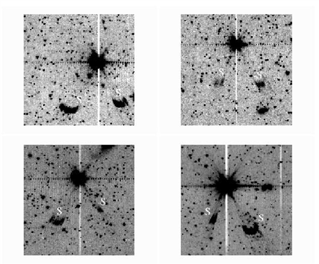
Figure 7.14: Channel 1 image showing scattered light on both sides of a bright star. The scattered light patches are marked with white “S” letters. The images were taken from PID=30 data.
Example images of scattered light are shown here to alert you in case you see something similar in your IRAC images. The scattered light pattern from point sources is difficult to predict, and very difficult to model for removal. To first order, you should not use data in which scattered light from point sources is expected to cover or appears to cover your scientific target. Stray light masking was done in the pipeline. This procedure incorporates our best understanding of the stray light producing regions. The procedure updated the corresponding imask for a BCD by determining whether a sufficiently bright star was in a stray light-producing region. The 2MASS point source list was used to determine the bright star positions.
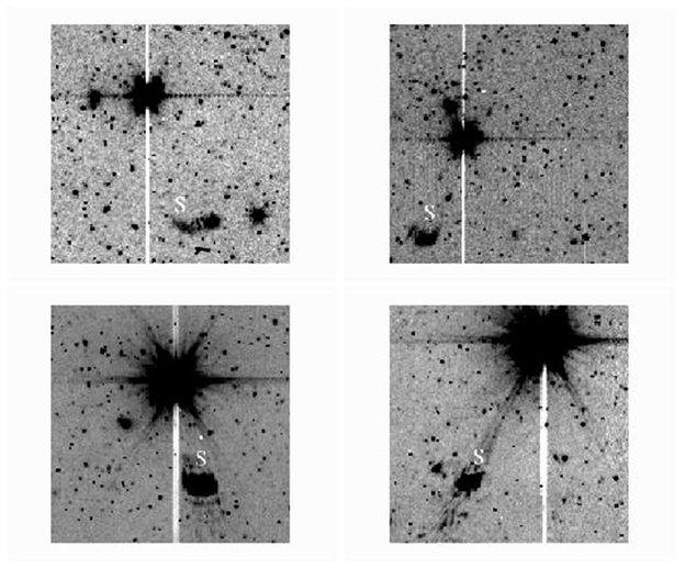
Figure 7.15: Similar to Figure 7.14 but for channel 2.
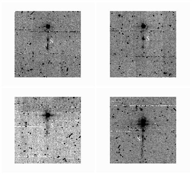
Figure 7.14 to Figure 7.17 are 201 pixels (4.1 arcminutes) square, and have been extracted from larger mosaics produced from the IRAC GTO shallow survey (from PID 30). This survey covered 9 square degrees with three 30-second images at each position. Because the mosaics cover large areas, the star causing the scattered light appears in many of the images. All of the sample images have the same array orientation as the BCD images. The sample images are mosaics of a BCD that contains the stray light and the BCD that contains the star that produces the stray light. Figure 7.14 and Figure 7.15 show scattered light in channels 1 and 2, from zones 1A, 1B, 2A, and 2B as identified in Figure 7.13. Figure 7.16 and Figure 7.17 show scattered light in channels 3 and 4. Because stars are much fainter in these channels, and the scattering geometry is much less favorable, these scattered light spots are much less obvious than in the short-wavelength channels. Dithering by more than a few pixels would take the bright star off the channel 3 and 4 “scattering strip,” so the scattered light spots should be removed from mosaics made with adequately dithered data.
Figure 7.16: Similar to Figure 7.14 but for channel 3.
Please note that Figure 7.14 – Figure 7.17 were made with no outlier rejection. A dithered observation, combined with outlier rejection, will have much reduced stray light. Further, a diligent data analyst, who recognizes and masks stray light in the individual BCDs, will be able to eliminate stray light from well-planned mosaics. Observations made with little or no redundancy, or with dithers on scales smaller than the size of the stray light patches, will contain stray light and should be used with caution. Information on how the pipeline masks suspected stray light areas is given in Section 5.2.1.
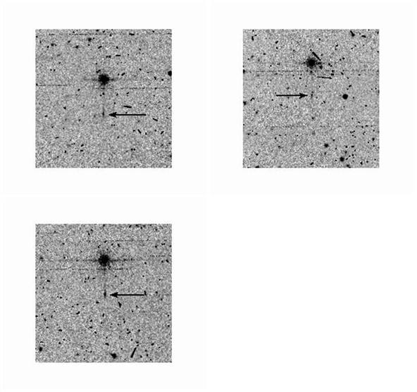
Figure 7.17: Similar to Figure 7.14 but for channel 4. The scattered light patches are pointed to by black arrows.
[2] We thank R. Arendt for providing us with most of the information that was presented in this section.