The goal of time series photometry is to produce a light curve of an astronomical source. The main challenge in producing light curves for systems whose intrinsic variations represent a small fraction (<1%) of the source average flux is to reduce or remove time-correlated noise and achieve photon-noise limited precision over all temporal binning scales. This section presents our best understanding of the sources of correlated noise and their mitigation, and recommendations for reducing time series data.
8.3.1 Time-Correlated Noise
Data reduction for time series is challenging due to both instrumental and astrophysical effects. This subsection focuses on the known instrumental effects which prevent observers from achieving Poisson noise limited light curves from IRAC data.
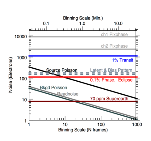
The relative strengths of instrumental systematics are shown in Figure 8.8 (Krick et al. 2016), and discussed in this section. We plot all known noise sources in units of electrons as a function of binned number of frames on the bottom and averaged minutes on the top, assuming 2 second frame times. This figure includes the Poisson contribution from an assumed source at half-full well as the solid diagonal black line, and the background noise, along with the readout noise, as the solid diagonal gray lines. The level of the intrapixel gain effect for both channel 1 and channel 2 are shown as the top horizontal gray lines (intrapixel gain effect is sometimes referred to as the “pixel phase” effect in literature and the effects for channels 1 and 2 are labeled “Pixphase” in the diagram). An estimate of the level of uncertainty caused by bias pattern effects and persistent images (latents) is indicated with dashed gray lines. We show the rough levels expected for a hot Jupiter transit, eclipse, and a 70 ppm super-Earth transit event.
The strongest instrumental effect in the warm mission IRAC is the under-sampled PSF coupled with gain variations within a single pixel, also known as the intrapixel gain (sensitivity) effect. When combined with random pointing fluctuations and systematic drifts, this becomes the largest source of noise in time-series measurements. In subsection 8.3.2 we discuss the ability of the Spitzer spacecraft to hold its position. A separate concern is pointing repeatability (subsection 8.3.3), where we have deliberately localized the pointing fluctuations to a single pixel. Once the spacecraft is able to repeatedly point to a single position, it was possible to map out intrapixel gain variations (subsection 8.3.4) for one particular pixel on each IRAC array. We review a number of additional potential sources of noise in time-series data, such as residual non-linearity (subsection 8.3.5), time-varying detector bias (subsection 8.3.6), pointing drifts (subsection 8.3.7), and persistent images (subsection 8.3.8). Techniques for removing correlated noise (subsection 8.3.9) are then discussed. We also address methods for measuring the improvement in photometry (subsection 8.3.10) achieved by removing correlated noise.
Figure 8.8: Noise in electrons as a function of binning scale showing the relative strength of instrument systematics. Noise contributions from the source and background are shown as diagonal lines. Known instrumental systematics are shown as horizontal lines. For reference, also shown are the strengths of a hot Jupiter (1%) transit, 0.1% eclipse, and a 70 ppm super-Earth transit.
8.3.2 Spacecraft Motion
Motion of a target across the detector array can be caused by spacecraft-induced motions including drifts, wobble, and jitter. Section 4.12 describes these effects in detail. Here we give a basic summary.
Settling drifts on the order of 0.5 arcseconds over the course of half an hour after slewing are thought to be due to variable heating and cooling within the spacecraft bus. The resulting small temperature changes cause very slight changes in the alignment between the star trackers and the boresight of the telescope. The temperature changes themselves are thought to be caused by heating of the spacecraft bus when the telescope is observing (or communicating with Earth) at relatively large pitch angles, and radiative cooling when the pitch angle returns to less than ±10 degrees. Depending on the amount of time spent at such high pitch angles, the spacecraft may require anywhere from hours to days to reach a temperature equilibrium.
On top of the initial settling drifts, there is a roughly constant, long-term drift (see Section 4.12.4.2) of 0.34 arcseconds per day in the y-pixel direction. This drift is thought to be due to an inconsistency in the way that velocity aberration corrections are handled by the spacecraft's Command and Data Handling computer (C&DH) and the star trackers. Whereas the C&DH assumes that velocity aberration is constant over the course of each AOR, the star trackers update the velocity aberration corrections continuously. The result is a constant error signal sent by the star trackers, for which the spacecraft constantly attempts to correct.
A second thermally-induced pointing drift is an oscillating “sawtooth” motion in both x- and y-pixel directions (also known as “wobble”; see Section 4.12.4.3). This is thought to be due to thermo-mechanical expansions and contractions of many of the same spacecraft components as above, motivated here by the periodic, on-off cycling of a battery heater within the spacecraft bus. The amplitude of the sawtooth was ≈ 0.15 arcseconds, with a period of about an hour. To reduce the amplitude of the oscillation and move the period away from the typical durations of exoplanet transits, the cycling range was reduced to 1 K on 17 October 2010. Data taken since that time show a sawtooth amplitude reduced by a factor of two, with a period of 39 ± 2 minutes.
Jitter (see Section 4.12.4.1) has both high frequency (> 50 Hz) and low frequency (≈ 0.01 Hz) components, with peak-to-peak amplitudes ranging from 0.03 to 0.1 arcseconds. Possible causes are many, and may include noise in the star tracker solutions, momentum variations in the reaction wheel assembly, harmonically coupled to the spacecraft structure, and even micrometeoroid impacts. High frequency jitter will presumably continue to set a noise floor for bright targets.
8.3.3 Repeatable Pointing
8.3.3.1 “Sweet Spot”
The first step towards reducing correlated noise is to localize the sub-pixel position of a point source on an area of minimal sensitivity (gain) variation. We have defined the “sweet spot” region of each array to be the 0.5-pixel square surrounding the point of maximum response in the subarray field of view center pixel (pixel [15,15] in [0,0]-based coordinates). Specifically, the sweet spot peak is at [15.198, 15.020] in channel 1 and [15.120, 15.085] in channel 2. To place the target on the sweet spot we used the PCRS function on Spitzer (see Section 3.2 for more information about the PCRS Peak-Up).
8.3.3.2 Why This Sweet Spot?
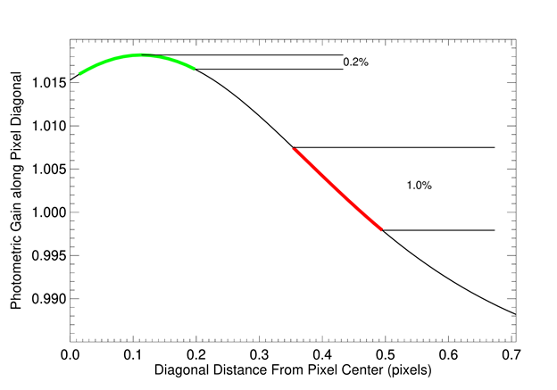
As shown in Figure 8.9, the peak pixel response in channel 2 is not at the center of the pixel. Also, note the 0.2% variation in gain around this peak for a typical pointing wobble, plus a drift of about 0.2 pixels, whereas the same motion would result in 1% gain variations closer to the corner of the pixel. Keeping a target within the sweet spot minimizes correlated noise.
Furthermore, the sweet spot of each array has been targeted by the IRAC team as a region for special calibration. Many thousands of photometric measurements of non-variable stars have been made in an effort to build a high spatial resolution, low noise map of intrapixel gain. Kernel regression techniques can be used to reduce correlated noise and provide an independent check on other noise reduction techniques.
Figure 8.9: Channel 2 photometric gain versus diagonal sub-pixel position, based on a crude Gaussian model of the pixel. The vertical ranges show the amount of gain variation over about 0.2 pixels at the peak of gain (green) and near the corner of the pixel (red).
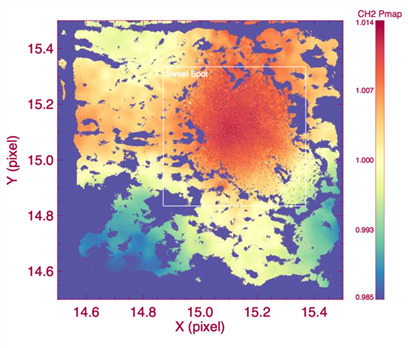
Figure 8.10: The map of intrapixel photometric gain, or “pmap” for channel 2 post-cryogenic data. This is the pmap built from data collected as of 2014/09/04. Note that gain is not symmetric around the center of the sweet spot and that the peak is not at the nominal center of the pixel.
8.3.4 Mapping Intrapixel Gain
Due to the undersampled nature of the PSF, the warm IRAC arrays show variations of as much as 8% in sensitivity as the center of the PSF moves across a pixel due to normal spacecraft motions. These intrapixel gain variations are the largest source of correlated noise in IRAC photometry. Many data reduction techniques rely on the science data themselves to remove the gain variations as a function of position. The IRAC team has generated a high-resolution gain map (called the “pmap”; see Figure 8.10) from standard star data, which can be used as an alternative when reducing data.
8.3.4.1 Centroiding
Finding accurate centroids for photometry is critical because it determines how much flux gets into the aperture. Systematic offsets from the measured centroid to the real centroid cause biases in photometry. Centroiding accuracy appears to be dependent on both the measurement technique and the geometric effects due to the location on the pixel. Measurement techniques include center of light, Gaussian fitting, and least asymmetry. The geometric effect of shifting flux into neighboring pixels generates the dependence on pixel location. If you are using the gain map provided by the IRAC team, it is important to use the same centroiding method (box_centroider.pro on IRSA’s Spitzer Contributed Software website, linked from irac_aphot_corr.pro) as was used for the gain map for consistency.
8.3.4.2 Noise Pixels
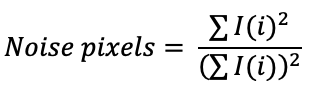
The number of noise pixels (see Section 2.2.2 for definition) is a measure of the apparent size of the image. Specifically, it is the equivalent number of pixels whose noise contributes to the flux of a point source. This quantity is useful as a parameter in removing the systematics of motion across a pixel over the course of a staring mode observation.
Summing over all pixels i, the intensity of each pixel is I(i), so that the noise pixel is the sum of the intensity squared divided by the sum of the squares of the intensity. The same measure can be split into its directional components, XFWHM and YFWHM.
(8.3)
(8.4)
(8.5)
These values do vary with the size of the regions used to do aperture photometry. If you are using these values with the gain map dataset, it is imperative that you calculate noise pixels and XFWHM and YFWHM in the same way as box_centroider.pro (available on IRSA’s Spitzer/IRAC web pages in the Calibration and Analysis Files section, warm mission intrapixel sensitivity corrections). That code uses an aperture radius of 3 pixels and a background of 3 - 7 pixels. Preliminary indications are that using the pmap with x, y, xyFWHM is not more effective than x, y, noise pixels.
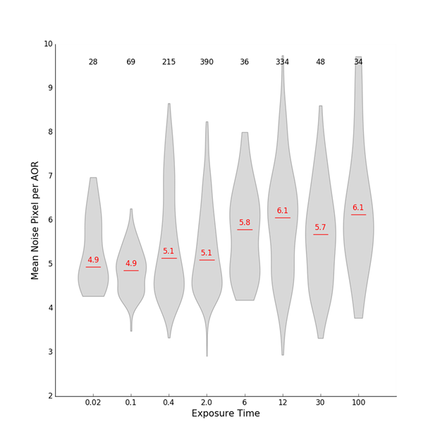
Noise pixel values have a range 4 - 8 depending on the location on the pixel, and which pixel the target falls on. There is no evidence that the PSF itself changed during the Spitzer mission.
We do see evidence for the number of noise pixels being correlated with exposure time (see Figure 8.11). Using all of the staring mode AORs in the warm mission archive through June 2017 (≈ 1300 AORs), we see a statistically significant change in noise pixels with exposure time.
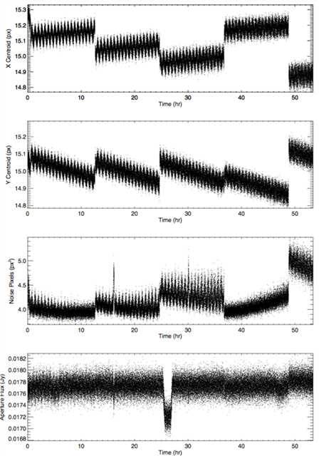
A few times over the course of the mission, the number of noise pixels has been seen to sharply increase in value for a short duration (≈ 30 minutes) before returning to normal (see Figure 8.12, at 16 and 30 hours). Figure 8.12 shows simulated data instead of archival data to demonstrate that we can successfully replicate noise pixel spikes, and therefore have a better understanding of their cause. See Appendix Section D.1.4 for a discussion of noise pixel spikes.
Figure 8.11: Distribution of average noise pixels per AOR vs. exposure time. All ≈ 1300 staring mode AORs from the warm mission through June 2017 were used. Each of the gray shapes represents the distribution for the corresponding exposure time. Red lines show the median value per exposure time and are marked with that median noise pixel value. The total number of AORs per exposure time bin is printed at the top of the plot. We use 3σ clipping to remove outliers, such as those that fell far away from the sweet spot.
Figure 8.12: x, y, noise pixels, and flux values as a function of time over five simulated AORs. Note the noise pixel spikes at 16 and 30 hours which are seen in the noise pixel and flux plots, but not in the x and y position plots. This simulated dataset is of WASP 52.
8.3.4.3 Optimal Aperture Size
There is an optimal aperture size to use which is bound on the small side by wanting to include enough target flux and on the large size by the exclusion of too much background noise. The optimal size varies from observation to observation and must be tested for each dataset.
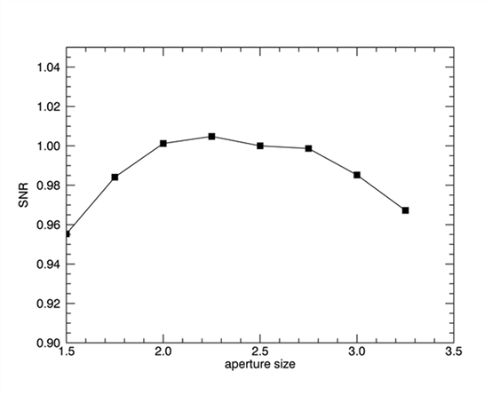
One way to determine the optimal aperture size is to look at a plot of signal-to-noise ratio (SNR) versus aperture size radius for a range of aperture sizes around the known FWHM of the IRAC PSF (≈ 1.7 pixels). It is also informative to look at a plot of just the noise as a function of aperture size. Figure 8.13 shows this for one example data set from the archive. A plot of sigma vs. aperture size is the inverse of Figure 8.13 where the noise decreases from aperture sizes 1.5 pixels until about 2 pixels, where it holds roughly steady until 2.75 pixel radius and then starts slowly increasing. We use gain map corrected SNRs, otherwise the uncertainties are dominated by the gain variations and not by the aperture size. In this case the signal is the mean corrected flux over the whole staring mode AOR, and the noise is the standard deviation of those corrected fluxes over the whole stare. The optimal aperture size for this target would be 2.25 pixels because that is where the SNR is highest and the uncertainties the lowest. Smaller aperture sizes do not include enough of the target star flux and larger aperture sizes include too much of the background and its associated uncertainty.
Figure 8.13: Signal-to-noise ratio versus aperture size for the WASP-14b exoplanet, normalized to an aperture size of 2.5 pixels in radius.
8.3.5 Residual Nonlinearity
In certain regimes, the IRAC detectors are nonlinear such that a given increase in the flux of incoming photons does not lead to a linear increase in the electron count rate measured by the detectors and electronics (see Section 2.3.2 for a discussion of IRAC detector linearity). The pipeline corrects for the effects of this nonlinearity on BCD pixel values, however, this correction is only good to 1%, depending on well depth. High precision photometry studies that want to use the gain map taken at one fluence (accumulated electron counts or well depth, often measured using analog-to-digital data number or DN at the pixel of peak response to a star; fluence in DN is proportional to the total electron counts) to correct science data taken potentially at another fluence level may be sensitive to variations in the uncorrected “residual nonlinearity.” We document the existence of this residual nonlinearity, and show that as long as the observations stay between 1000 and 15000 DN (in channel 2), it does not seriously affect flux as a function of position on the pixel.
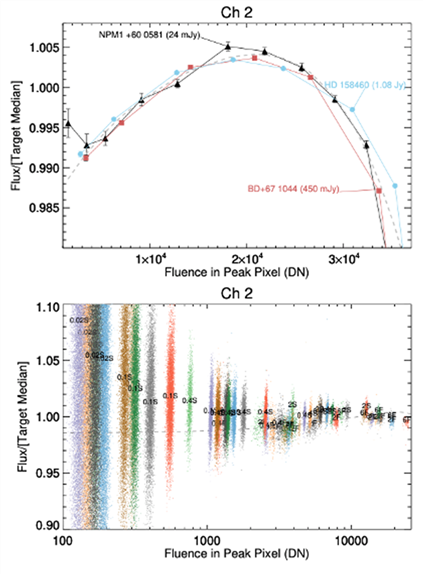
On both panels of Figure 8.14 we see a nonlinear relation between the amount of input counts (DN) and the measured flux. These are two different data sets that were designed to look at this relation by changing either the exposure time on the same star using IERs (a) or changing the exposure times on a set of stars using AORs (b). Both datasets have already been corrected by the pipeline nonlinearity. Anything that is not a flat line in these plots is a residual nonlinearity.
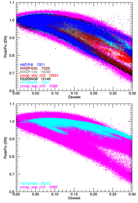
However, the existence of residual nonlinearity does not appear to affect the shape of the gain map (pmap) as a function of gain. We show this as a plot of peak pixels in DN vs. distance from the center of the sweet spot (Dsweet; Figure 8.15). The DN in the peak pixel decreases, as expected, with larger distance from the center of the sweet spot. The shape of this falloff is not symmetric around the center, and therefore leads to an envelope of points in Figure 8.15. Each color in this plot represents a different star with a different peak pixel DN level, where each star has been normalized to the center of the sweet spot. The fact that these envelopes are all of the same shape and overlap on the normalized plot indicates that the pmap does not have a different shape depending on DN. Therefore, residual nonlinearity does exist, but is not changing the shape of the pmap.
This probably works because most of the stars tested in Figure 8.15 have DNs in the range of 10000 to 25000 where the Fowler-sampled count rates have been sufficiently linearized. As seen in Figure 8.14, the slope of residual nonlinearity does not change for this range of DNs. That slope is already incorporated into the pmap because the pmap star has a source DN which varies significantly as a function of position, so the pmap is made with some degree of residual nonlinearity built into it. This makes the shape of the gain map the same for all the DNs in the “good” range.
Proof that this is a good plot to use to understand the effect of the residual nonlinearity comes in the second part of Figure 8.15. To see this best, we have plotted only the pmap 3000 DN observations and HD 158460 28000 DN observations. The observations at 28000 DN have a different slope to the top envelope that we do not see in any of the other observations in the more linear regime.
These results imply several things. First, the gain map can be used to correct photometry in the good DN range. Second, pixel level decorrelation (PLD) can be used with the gain map dataset coefficients to correct other photometry in the good DN range. Third, it should be ok to add other datasets to the gain map data set to fill in coverage, although this has not been tested. And fourth, distance from the sweet spot should be used carefully in all analysis tasks.
Figure 8.14: Residual nonlinearity in warm mission channel 2 data. These plots show linearity-corrected aperture flux as a function of well depth (fluence) for a set of targets, measured on the “sweet spot” of Channel 2. Top: binned aperture flux measurements of three targets, normalized to the median of each target. Well depth was varied using instrument engineering requests (IERs) to vary the frame time and corrected with special dark frames obtained the same way. Data were binned by frame time. A 4th order polynomial fit to the data is overlaid as a dashed curve. Names of the stars are labeled, along with average flux densities. Bottom: Unbinned aperture flux vs. fluence data for 15 additional stars measured using AORs, color-coded by star. Frame times are labeled (in seconds) at the location of the median flux and fluence for a given frame time and star, with the qualifier “S” or “F” to denote full or sub-array readout mode. For comparison, we have overlaid the fit from the top plot. Measurements with perfectly corrected nonlinearity should lie on a straight horizontal line.
Figure 8.15: Peak pixel value in DN vs. distance from the sweet spot in channel 2. Sweet spot is defined here to be [15.12, 15.1] (when [0,0] is defined as the bottom left corner). These stars are all observed with multiple snapshots, and include the gain map calibration star itself taken with two different frame times. The second plot shows the different slope when using a 28 K source.
8.3.6 Time-varying Bias in Point Source Data
8.3.6.1 Staring Mode Darks
Observations taken with a dither pattern will have a different bias level and pattern than observations taken in staring mode. This is because the bias is sensitively dependent on both the time between observations, and all previous observations. The dither pattern is important because the frame delay times are determined by the slew times inside of that pattern. The delay time is at least seven seconds between pointings for dithered observations (includes slewing), but only about two seconds between successive staring frames, and within a 64-frame subarray, there will be 0 seconds frame delay.
This is relevant to light curve staring mode photometry because the IRAC pipeline uses an image of the dark current which is made from dithered observations to remove the bias pattern from all observations, regardless of dithering or staring. Because IRAC did not use a shutter, an image of the dark current was generated by making weekly observations of a relatively blank region of the sky at the north ecliptic pole (NEP). When this dithered dark observation was used to correct a staring mode observation, there was the potential for a low-level bias pattern residual in the dataset. This residual pattern could affect the photometry of staring mode observations. The inaccuracy in the bias level (as opposed to pattern) does not matter for aperture photometry.
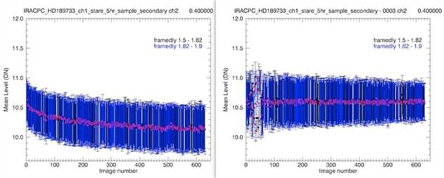
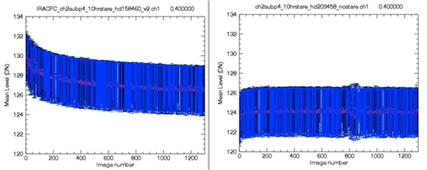
IRAC data do have a change in inter-frame delay times over the 64 subframes of a single BCD, since the first sub-frame will have a longer delay time than the subsequent sub-frames. We have also seen evidence in archival data of a bias level change over the course of long (5 - 10 hour) stares (see Figure 8.16), which leaves open the possibility that there is also a bias pattern change on those timescales.
To explore these bias patterns, the IRAC team designed and executed test observations of the NEP field with the staring mode. Our goal with these observations was to measure the difference between dithered and staring mode darks at the frame times which are useful for high precision staring mode photometry, and to determine the necessity and feasibility of using staring mode darks on staring mode observations. Please see Section 4.8 for more information on the recommended staring mode skydarks.
8.3.6.2 Superdarks
IRAC dark taking procedure is summarized in Section 4.1 and Section 5.1.15. Note specifically that for each science frame, the nearest-in-time skydark was used to correct that frame. The advantage of this weekly dark is that it removes any low-level persistent images which may be present in the science frames.
This means that a) different darks are used for different observations of the gain map since that dataset was observed over many years, and b) for datasets that use the gain map, different dark frames are subtracted from the gain map than are subtracted from target observations.
We tested the use of different darks in the gain map data set by first generating a superdark frame and then applying it to all the data frames of the same frame time. The superdark was generated by median-combining all dark images taken during the warm mission of a single frame time. The median-combine will reject all sources since these data were taken on-sky. The background level of the dark frames taken at the north ecliptic pole will vary as a function of time, but since most users are doing aperture photometry, and not absolute photometry, we do not care that the mean level of the dark is incorrect by the amount that the zodiacal light fluctuates over a year. The superdark is applied to each data frame by first backing out the calibrations already applied to the BCD, including the weekly dark, and then calibrating those images with our superdark.
We tested the superdark versus weekly dark in the gain map calibration star data set by testing both versions in a set of ≈ 30 different AORs taken on a different calibration star. We saw lower scatter in the observations taken with the weekly dark. Therefore, we did not use the superdarks in our current gain map dataset. The cause for this difference in scatter is likely to be local in time persistent images in the science frames which the local darks were able to partially mitigate, whereas the superdarks did not.
Figure 8.16: Bias Level in DN as a function of time. Bias level changes on long time scales (≈ 10 hours). Bias level as a function of time appears to not be repeatable from AOR to AOR. The data set used to make these plots consists of ten serendipitous staring mode AORs (five in each channel, 0.4 second frame time) in the off-field position, so theoretically empty of stars, although there are some stars in these observations. This bias change is not dependent on the frame delay (all frame delays show the change as a function of time). From these five AORs per channel, the maximum deviation is ≈ 2 DN in channel 1 and ≈ 0.5 DN in channel 2. These are binned over the whole BCD, so each point includes the mean from all 64 subframes. Only one amplifier is shown. Blue and black points show the different frame delays, for which there is no correlation with the shape of the long time scale change. Here we show two plots for each channel to demonstrate the range of level changes.
8.3.7 IRAC’s Photometric Stability
We examined the photometric stability of the IRAC detectors as a function of time over the course of the first 11 years. This is relevant to high-precision time-series photometry in considering the use of the pixel phase gain map to correct data sets which were not taken contemporaneously with the gain map dataset. The data for the gain map itself were taken over the course of more than one year, and will consequently also be affected by instabilities in photometry over year-long timescales.
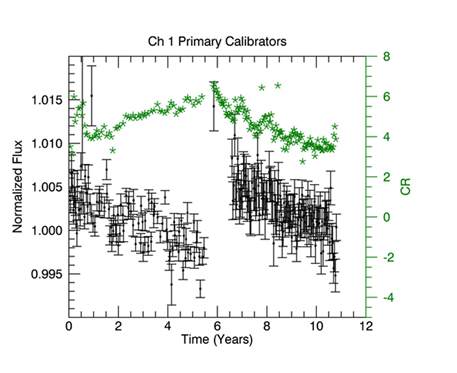
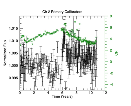
We used the primary calibrators to examine photometric stability. The data set consists of A and K stars, known to be stable at these wavelengths, observed roughly every two weeks throughout the mission. Figure 8.17 shows aperture photometry of seven calibration stars observed with a dither pattern in full array, binned together on two-week timescales. Photometry is corrected for both the array location dependence and pixel phase effect using a double Gaussian approximation to the pixel phase effect. Dithering to many positions and binning over all stars will reduce systematics from each of these effects. Each individual star is normalized to its median cryogenic mission level before being binned together with the other calibration stars. Error bars show the 1σ standard deviation on the mean divided by the square root of the number of data points in the bin. The cryogenic mission has more data points per bin, but a lower frequency of observations since the instrument was not always in use, accounting for the smaller cryogenic mission error bars.
Data from the end of the cryogenic mission to about nine months into warm mission was processed with a different flux conversion value, and the fluxes are therefore offset for that time period. In channel 1 they are not even within the axis range plotted, which causes the gap in the plot at about six years. The offset in normalized flux from the cryogenic to warm mission is likely caused by the fact that flux conversions are determined from the entire dataset without regard to this measured slope. Taken as an ensemble, the cryogenic and warm mission flux conversions are designed to be consistent. The channel 2 data set is noisier because the stars have a lower signal-to-noise ratio (the same star is fainter in channel 2 than in channel 1).
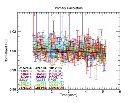
Individual light curves for each of the calibration stars used in this analysis were checked to rule out the hypothesis that one or two of the stars varied in a way as to be the sole cause of the measured decrease in binned flux as a function of time. This is shown in Figure 8.18 for the channel 1 warm dataset, with each star represented by a different color. Slopes and their chi-squared fits as well as the star names are printed on the plot. While the slope for each individual star is not as well measured as for the ensemble of stars, it is apparent that the decreasing trend is seen in all or most stars, and is not caused by outliers.
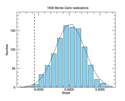
There is a statistically significant decrease in the sensitivity of both channel 1 and channel 2 over the course of the mission. The deviation from zero change, a flat line fit to the data as a function of time, is tested using a Monte Carlo techniques. We ran 1000 instances, randomly shuffling the order of the times associated with each flux bin. The resulting distribution of the measured slope is consistent with a Gaussian distribution around a zero slope, and is not consistent with the slopes measured here in the sense that > 95% of the instances have slopes closer to zero than what the calibration star data show. This is shown in the blue histogram in Figure 8.19 for the channel 2 warm data sets. The dashed line shows the measured slope.
One hypothesis as to the cause of the decrease in flux over time is the decrease in cosmic rays (CR) hits over time due to the solar cycle. Green points show the CR counts taken from the 100 second north ecliptic pole fields. Solar minimum occurs around the changeover between the cryogenic and warm missions. Solar maximum was around 2014, 11 years into the mission. CR counts should decrease as the solar activity increases because the solar activity pushes the volume of solar influence further out, which decreases the number of CRs that reach Spitzer. Since we see both CR counts increasing and decreasing over the mission, whereas the fluxes always decrease, the solar cycle cannot be the cause of the flux decrease.
The decrease in sensitivity is potentially caused by radiation damage to the optics. The decrease in sensitivity is different for the two channels, with the slope of the change being steeper for channel 1.
What are the implications of this for science? The degradation is of the order of 0.1% per year in channel 1 and 0.05% per year in channel 2. These levels are only relevant to high precision studies. Relative photometry studies will be immune to such changes since all the photometry will change equally. Similarly, measurements of transit and eclipse depths will not change as a function of time due to this effect because they are measured relative to the rest of the light curve.
Figure 8.17: Channel 1 and 2 ensembles of primary calibrator fluxes as a function of time since the start of the mission. Black points show the ensemble of primary calibrators while green stars show the cosmic ray counts.
Figure 8.18: Individual calibration stars as a function of time. There is no evidence for a single outlier star as the source of the flux degradation trend.
Figure 8.19: A Monte Carlo simulation of calibration flux vs. time stamp slopes. This figure shows what the slopes would be if the time stamps for each data point were shuffled using a Fisher - Yates shuffle. The actual measured slope for channel 2 is shown with the dashed line. Because this measured slope is outside of 1σ, we take the slope to be significant.
8.3.8 Persistent Images
Persistent or residual images are discussed in Section 7.2.8. Both IRAC channels 1 and 2 sometimes show residual images of a source after it has been moved off a pixel. Beyond intrapixel gain effects, we expect these persistent images to be the next largest source of noise in multi-epoch high precision photometry observations. When a pixel is illuminated, a small fraction of the photoelectrons are trapped. The traps have characteristic decay rates, and can release a hole or electron that accumulates on the integrating node long after the illumination has ceased. Persistent images on the IRAC array start out as positive flux remaining after a bright source has been observed. At some later point in time the residual images turn from positive to negative, so that they are actually below the background level (trapping a hole instead of trapping an electron). Positive and negative persistent images in either the aperture or background annulus in either the dark frame or the science frames can lead to artificial increases or decreases in aperture photometry fluxes. Persistent images are pervasive. We will use the terms persistent images and residual images interchangeably throughout this discussion.
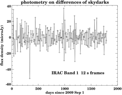
Short-term persistent images start at about 1% of the source flux and can be seen to decay over the course of minutes to hours. While some patterns change weekly, some persist over multiple weeks. We show a plot in Figure 8.20 of the change in photometry on a blank region in difference images for the channel 112-second frame time. Using the size of the fluctuations in the blank sky photometry, we then calculate the percentage effect that the residual images have on photometry which is shown for all frame times and both channels in Table 8.3 below. The apparent pinging back and forth from week to week at the level of 10 - 15 μJy is likely due to the “first-frame effect” because of the way that the skydarks are observed. Residual images have a much stronger effect in channel 1 than in channel 2, and are strongest at 0.4 and 2 second subarray frame times.
Beyond knowing of their existence, it is very difficult to quantify these low-level latent images, especially since we know that the residual images are both growing with new observations dependent on the specific observing history, and shrinking over time as they dissipate. Our superdark analysis shows that persistent images can affect photometry at the 0.1% level (see Figure 8.20).
Figure 8.20: Skydark variations in channel 1 over the course of the warm mission. The y-axis is a difference of the flux density present in the darks after an average dark frame has been removed.
Table 8.3: Approximate levels of the residual fluxes as a function of channel and frame time.
Frame time (seconds)
Channel 1 sigma (%)
Channel 2 sigma (%)
0.02 sub
0.03
0.01
0.1 sub
0.07
0.01
0.4 sub
0.1
0.02
2 sub
0.11
0.03
0.4 full
0.06
0.05
2 full
0.06
0.04
6 full
0.07
0.03
12 full
0.07
0.04
8.3.9 Removing Correlated Noise – Repeatability and Accuracy
There are several techniques in the literature for removing correlated noise from IRAC high precision photometry data sets. Please refer to the following papers as starting points for a discussion of those techniques.
BiLinearly Interpolated Subpixel Sensitivity (BLISS; Stevenson et al. 2012)*
Kernel Regression Mapping, using the data to be corrected (KR/Data; Ballard et al. 2010, Knutson et al. 2012)*
Gaussian Process Models (GP; Evans et al. 2015)*
Independent Component Analysis (ICA; Morello et al. 2015)*
MCMC Evaluation (Gillon et al. 2010)
Pixel Level Decorrelation (PLD; Deming et al., 2015)*
Kernel Regression using a calibration pixel mapping dataset (KR/Pmap; Krick et al. 2016)*
Polynomial fitting (Charbonneau et al. 2008)
Segmented Polynomial for the K2 Pipeline [SP(K2)] ( (Buzasi, D. L. et al, 2015))*
*Methods compared in FiguresFigure 8.21 and Figure 8.22.
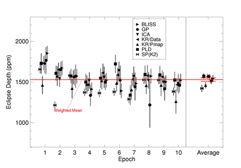
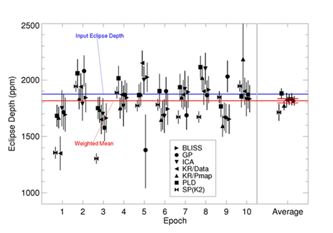
Ingalls et al. (2016) examined the repeatability, reliability, and accuracy of differential exoplanet eclipse depth measurements made using IRAC during the warm mission. The authors re-analyzed an existing 4.5 μm data set, consisting of ten observations of the XO-3b system during the secondary eclipse, using seven different techniques for removing correlated noise. They found that, on average, for a given technique the eclipse depth estimate is repeatable from epoch to epoch to within 150 parts per million (ppm; see Figure 8.21). Most techniques derive eclipse depths that do not vary by more than a factor of three of the photon noise limit. All methods but one accurately assess their own errors: for these methods the individual measurement uncertainties are comparable to the scatter in eclipse depths over the ten-epoch sample. To assess the accuracy of the techniques as well as to clarify the difference between instrumental and other sources of measurement error, the authors also analyzed a simulated data set of ten visits to XO-3b, for which the eclipse depth is known (Figure 8.22). They found that three of the methods (BLISS mapping, Pixel Level Decorrelation, and Independent Component Analysis) obtain results that are within three times the photon limit of the true eclipse depth. When averaged over the ten-epoch ensemble, five out of seven techniques come within 100 ppm of the true value. Spitzer exoplanet data, if measured following best practices and reduced using methods such as those described, can measure repeatable and accurate single eclipse depths, with close to photon-limited results.
Figure 8.21: Eclipse depths for ten visits to XO-3b, as computed via various methods. The group of points for each epoch is separated to minimize confusion. Error bars in this plot are symmetric; in cases where the technique returned asymmetric uncertainties, we used the largest of the two values. We show the results for the separate visits to the left of the gray vertical line, and the average results to the right. Error bars on the separate visits are the uncertainties reported by the technique. Error bars on the averages are the uncertainties in the weighted mean, adjusted for “underdispersion” using the scatter in the group of measurements. The horizontal red lines display the grand mean for all the results, and its uncertainty.
Figure 8.22: Similar to Figure 8.21. A blue horizontal line indicates the eclipse depth input to the simulations, 1875 ppm.
8.3.10 Measuring Noise Reduction
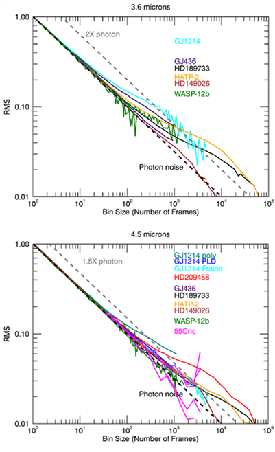
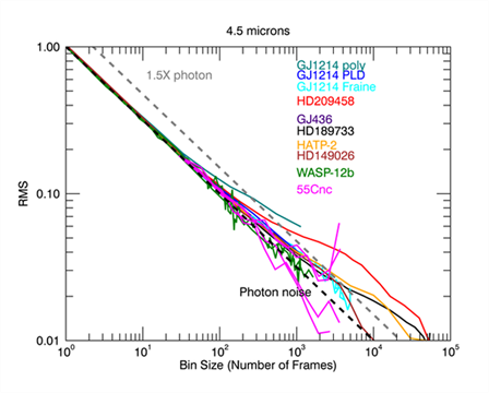
We explore how well any given IRAC data reduction has removed the above sources of correlated noise. It is challenging to remove systematics without removing time-varying astrophysical signal. One possible metric of the final achieved precision is to examine the RMS as a function of binning scale and compare that to the photon noise limit. References to the data presented in Figure 8.23 are HD 189733 (Knutson et al.,2012); GJ 436 (Knutson et al. 2011); GJ 1214 (Fraine et al. 2013); HD 209458 (Zellem et al. 2014); HD 149026 (Stevenson et al. 2012); HAT-P-2 (Lewis et al. 2013); WASP-12 (Stevenson et al. 2014); and 55 Cnc (Demory et al. 2016).
Figure 8.23: Actual precision reached for published, single epoch, IRAC observations. Plots are normalized at a binning size of one. The dashed black line is photon noise limited. The dashed grey line is two (1.5) times the photon noise limit for channel 1 (2). The third plot is a zoom-in on channel 2.