FORCAST Imaging Observing Modes - This document provides an overview of the imaging modes available with FORCAST.
FORCAST Grism Observing Modes - This document provides an overview of the grism observing modes available with FORCAST.
This page will cover the following topics:
- 1. FORCAST SSpot AOR Checklist
- 2. FORCAST Imaging Observations
- 3. FORCAST Spectroscopic Observations
- 4. Other Important AOR Issues
Other help:
- The FORCAST instrument page and the FORCAST section of the Cycle 4 Observer's Handbook give further details of the instrument's capabilities
- Further details on general (non-FORCAST specific) SSpot functionality can be found in the SSpot Pocket Guide and in the SSpot User Guide .
- For questions not answered by any of this material, please contact the SOFIA help-desk
FORCAST Phase II Preparation for Cycle 4
During Cycle 4, the FORCAST support scientists will be generating the first draft of the AORs for each program. Once the first drafts are complete, the GIs will be notified by their support scientists that their AORs will be available for review. GIs should work directly with their support scientists to make necessary changes to their AORs according to the information provided here.
1. FORCAST SSpot AOR Checklist
To speed acceptance of your Phase 2 AORs, you may wish to consider the following checklist.
- Did you check to make sure that you are chopping and nodding on to clean sky? All observations should be checked by looking at WISE, Spitzer, MSX, or IRAS images first to make sure that the chopping and nodding configurations are set up properly.
- Does your source fit within the field of view of FORCAST given any rotation of field (i.e. your object must not be any bigger than 3.2' across in any dimension)? If yes, are you chopping far enough so that you are chopping off of your source? If no, have you specified your mosaic strategy ?
- Did you prioritize your targets if you have some that are more important to observe than others? Make sure you have set up your Observing Priority . Very importantly, make sure ALL observations (AORs) for a particular target have the same Observing Priority.
- Did you prioritize the individual observations (AORs) for each target? Make sure you have set up your preferred observation Order .
- Did you provide comments for non-standard observations or special requests?
- If you are using C2NC2 or NXCAC mode with a chop throw >250", did you specify as large a range of chop angles as you could?
- For the imaging or spectroscopy of extended and bright sources, did you set up dithers to mitigate array artifacts?
- For imaging mosaics of extended objects larger than the FORCAST field of view, did you set up the mosaic offsets so that there is adequate overlap so that there will be no gaps in coverage regardless of the sky orientation at the time of observation? You may wish to consult the information on mosaicking .
2. FORCAST Imaging Observations
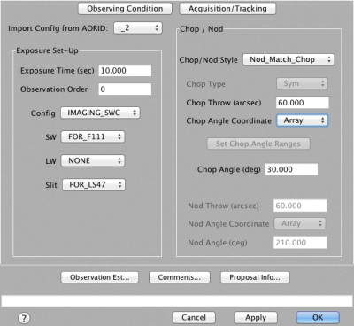
2.1. Setting the Instrument Parameters for Imaging Observations The majority of sources imaged with FORCAST will be relatively compact (source diameters <120") and lie in areas of the sky free from contaminating extended emission. For such observations, using the Nod-Match-Chop (NMC) imaging mode is recommended. Because coma will increase with larger chop throw (1" of coma for every 60" of chop throw in NMC), the chop throws should be configured to be as small as possible, but large enough that they know they will be chopping off source and onto clean sky. If there are clear chop reference areas all around the science source, then NMC mode should be configured with a chop angle of 30 degrees (which mitigates problems due to array artifacts) in the "Array" chop angle coordinate system.
If the source is surrounded by extended emission, the GI will have to configure the chop throw and angle in the "Sky" chop angle coordinate system to avoid contamination in the chop reference fields. This is discussed in more detail and with examples below ( Section 2.3 ) . This is also where you will find a discussion of using the C2NC2 mode for imaging very large and extended objects.
The GI also may or may not wish to dither the observations. Section 2.4 discusses the general rules of thumb for dithering with FORCAST.
2.2.Setting the Chop/Nod Parameters for Imaging Observations
The desired total on-source integration time should be determined by using the SITE on-line calculator and entered into the "Exposure Time" field. This value does not include overheads. The basic layout of the SSpot imaging panel is shown in the figure below.
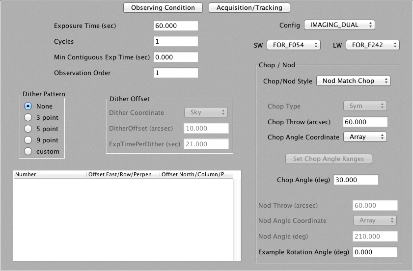
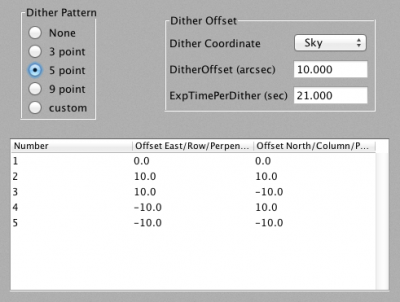
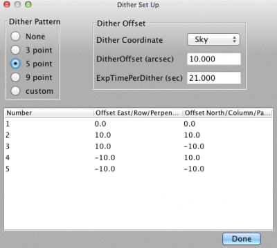
If you have a compact or faint source and are using the default NMC chop/nod mode, it is recommended that you do not employ dithers in your observation. This means you will not want to change your AOR from the default configuration where Dither Pattern is set to No. If you are not dithering, you can place the on-source integration time from SITE in the field marked “Exposure Time (sec)”. If you have an extended source and are using the default NMC chop/nod mode, or if you have another reason to do so, you may wish to dither your observations. There are two possible approaches to conducting dithered observations - you can step through each position in the dither pattern once until the pattern is complete, or the dither pattern can be looped through multiple times until the total on-source time is achieved. For NMC mode, it is better to only loop through the dither pattern once as this minimizes the overheads associated with the observation (and maximizes the observing efficiency, as we will see in an example below). In some cases, however, you may desire to loop through the dither pattern multiple times to build your desired total on-source exposure time (though we discourage doing this in NMC mode). In either case, the GI will select the desired pattern in the “Dithern Pattern” box of the main AOR panel. This will update the dither offset parameters to the default values for a pattern with the selected number of positions. The GI can also define the dither offsets and whether to do these offsets in RA and Dec (Dither Coordinates = “Sky”) or in x and y pixel coordinates (Dither Coordinates = “Array”). An example is shown in the image below.
If you are going to be dithering only once through the pattern, then you will have to divide the desired total on-source integration time by the number of dithers and put this value in the “ExpTimePerDither (sec)” field. This will automatically update the "Exposure Time" field with the total on-source time. Likewise, if you wish to repeat the dither pattern multiple times, then you will need to divide the desired total on-source integration time by the number of dithers PLUS the number of times you wish to repeat the pattern. You then specify the number of times you wish to repeat the dither pattern in the "Cycles" field. SSPOT calculates the actual duration of your observations based upon the chop-nod mode selected, the exposure time, the number of dithers, and the number of cycles. Pressing the “Observation Est.” button on the bottom of the main AOR panel will launch an information window that tells you the total requested exposure time, the overhead, and the duration of the observation. One can therefore check the observation efficiency by configuring the observations and pressing this button. For example, if you set up the AOR in NMC to have a 3-point dither pattern, with an exposure time of 60s per dither position, and one cycle, the resultant total exposure time will be 180s and the duration of the observation will be 425s (including estimates for line-of-sight (LOS) rewinds). If you set up an AOR in NMC with a 9-point dither pattern with an exposure time of 10s per dither and two cycles, the resultant total on-source exposure time is still 180s, but the observation will take 878s (almost twice as long). Since GIs are awarded time in duration, not exposure time, it is in the GI’s best interest to figure out how to use that time most efficiently. Note too, that when one specifies multiple "Cycles", that the "Exposure Time" field only displays the on-source time for a single cycle. The total on-source exposure time is displayed in the "Observation Est." window.
If you are using the C2NC2 chop/nod mode, then you are REQUIRED to specify dithers in your AOR. In the case of C2NC2 observations, you will likely need to loop through the dither pattern multiple times to build your desired total on-source exposure time. This is because the maximum allowed exposure time per dither is 21s if you are using the IMG_SWC or IMG_DUAL instrument configuration, or 63s if you are using the IMG_LWC instrument configuration. Furthermore, though it is possible to specify any number of dithers using the "custom" dither patter, the maximum number of dithers is 10 in C2NC2 mode. Therefore, if you need to observe a target with an exposure time longer than 210s in IMG_SWC or IMG_DUAL mode, or 630s in IMG_LWC mode, you will need to use multiple cycles through the dither pattern to build your total exposure time. The GI first sets the "Chop/Nod Style" in the Chop/Nod parameters box of the main AOR panel to "C2NC2". They then need to select the number of dither positions and their offsets (Dither Coordinates =“Sky” is the only option for C2NC2 mode) If cycling through the dither pattern only once, then the “ExpTimePerDither (sec)” field will be equal to the desired total on-source integration time divided by the number of dithers. The value now displayed in the “Exposure Time (sec)” field should have automatically been updated to the total desired on-source exposure time. If the dither pattern is to be repeated, then divide the desired total on-source integration time by the number of dithers PLUS the number of times you wish to repeat the pattern. This value is then input into the “ExpTimePerDither (sec)” field. Then specify the number of times you wish to repeat the dither pattern in the “Cycles” field. The value now showing in the “ExpTimePerDither (sec)” field multiplied by the value entered into the “Cycles” field should add up to the total on-source exposure time you desire.
2.2.3 Minimum Contiguous Exposure Time
In some cases, it is necessary to split an observation among multiple flight legs. The "Min Contiguous Exp Time" field should be used to provide flight planners with information on the minimum on-source exposure time that can be scheduled for a single flight leg to be scientifically useful. For example, if a program has been awarded 2 hours of time for imaging a faint target, it may be necessary to divide the observation over multiple flight legs. If the source is faint enough to require at least 45 minutes of on-source time in order to be able to accurately coadd the data from multiple flight legs, then this should be entered into the "Min Contiguous Exp Time" field.
The GI must then select the appropriate instrument configuration and filters for the AOR. All of the available FORCAST filters are listed, but there are some important considerations that must be made. First, the throughput with the 5.4 and 5.6 μm filters in Dual Channel mode is very poor. Thus, GIs are discouraged from using these filters in Dual Channel mode unless they are observing a blue source. Second, though all of the filters available for use in FORCAST are listed, only 12 are available in the instrument during any single flight series. As stated in the Call for Proposals filters that are not included in the non-standard filter set may not be available. If a program that includes non-standard filters has been awarded time, then the GI should contact their support scientist directly to determine if the non-standard filters will be available during the period when the program is scheduled. If not, then alternative filters must be used. The nominal filter set for SWC includes 6.4, 6.6, 7.7, 11.1, 19.7, and 25.3 μm. The supplemental filter set includes 5.4, 5.6, 8.6, 11.3, 11.8, and 24.2 μm. For LWC, the default filter set includes 31.5, 33.6, 34.8, and 37.1μm, while the supplemental set includes the 24.2 and 25.4 μm filters.
2.3. Observing Extended Objects Larger than the FOCAST FOV
In some cases, the target of interest will be quite large. Chopping beyond about 180", the imaged sources will have significant coma (>3"). The GI may wish to use the C2NC2 mode of observing in these cases. The C2NC2 mode allows for chop throws of up to 420” and yields images with no coma, however these observations are much less efficient (almost 2 times longer duration than C2N modes), so if you were awarded time for your observations under the assumption that NMC or NPC mode would be used but you find during Phase II that you will require C2NC2, then you will have to observe with fewer filters or observe less targets to still fit the C2NC2 observations within the awarded time.
The GI may wish to image an area much larger than the FORCAST FOV by creating a mosaic. Any mosaic with both dimensions larger than the FORCAST field of view should also be set up in C2NC2 mode (given the constraints on image quality due to coma when using large chop throws in NMC imaging mode). At present, there is no mapping mode available to create a mosaic automatically. Instead, the GI must specify the RA and Dec coordinates for each position of the mosaic manually and enter them as independent targets; (and, consequently, independent AORs). However, keep in mind that the GI cannot control the field orientation on the sky. This is determined by the object's position in the sky during the observing leg (i.e., by the flight plan), and this is not known until the specific observing leg is planned by the flight planners. For example, in the image below, the C2NC2 mosaic observations have been defined so that the target fields to be mosaicked are barely overlapping, thus maximizing the area sampled (the chop angle is defined as 110 degrees and is shown in green for each position; the nod B fields are not shown):
However, if the actual sky orientation is 45 degrees different from this in flight, the GI may end up with a mosaic with large coverage gaps:
The positions should be specified close enough to one another that they will overlap for ANY field orientation, allowing the GI to combine them into an uninterrupted map in the post-processing stages. This can be tested by changing the "Example Rotation Angle" in the AORs and reloading the AORs into the visualizer.
In order to freeze the target field on the detector, the telescope must rotate about its optical axis during an observation (SOFIA and FORCAST do not have image rotators). Because of the construction of the telescope, there is a limit to the amount the telescope can rotate. This limit is +/- 3 degrees. Once the telescope reaches this limit, the observation must be stopped and the rotation angle of the telescope is reset (a.k.a., an LOS rewind ). Then the source is reaquired and a new observation is started. The speed of the field rotation is set by the loaction of the object in the sky and the location of the aircraft. Because of the rotation limit, long integrations or observation of sources in parts of the sky that rotate quickly, may need to be broken up into several observations, each of which will have a different rotation angle.
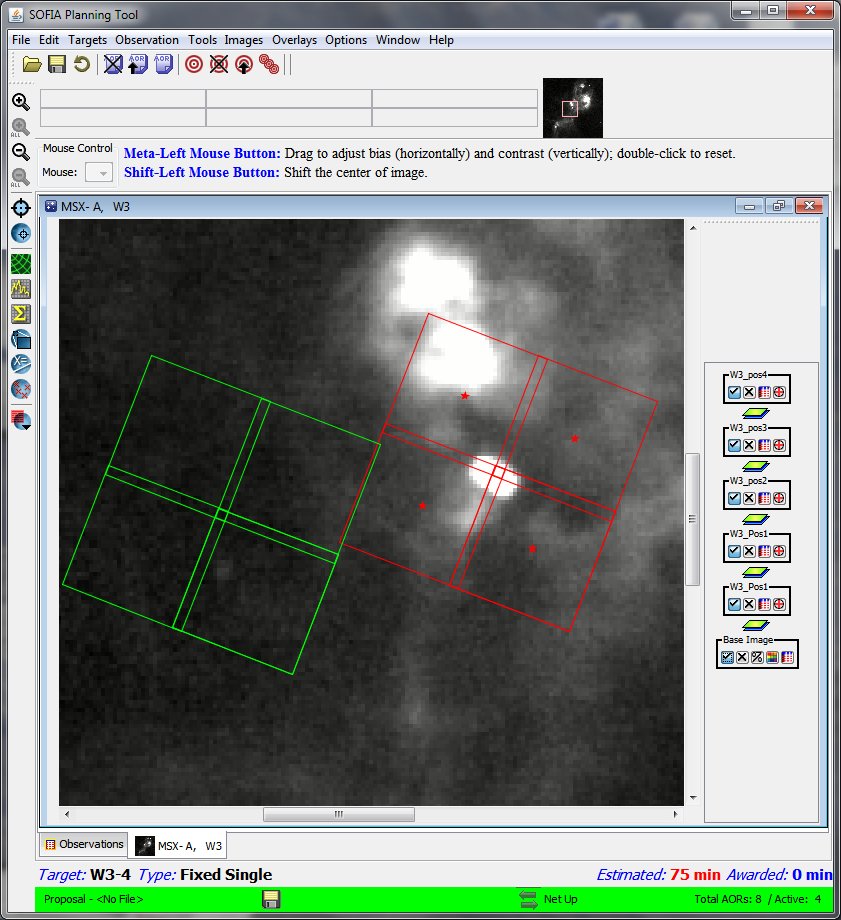
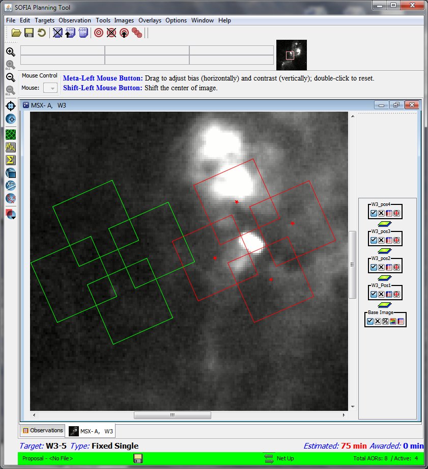
Therefore, for long integrations, or for sources in parts of the sky that rotate fast, the GI may expect that different elements of their mosaic may sample the source at different position angles. An example of this with a mosaic of W3 is shown below. Again the chop/nod mode is set to C2NC2 and the field of interest is being mapped by the red boxes. The chop angle is defined as 110 degrees and is shown in green for each position. As in the previous example, in this example the chop angle and throw were both kept the same for each element of the mosaic since there was adequate emission free space available near the science target, but the same nod position was used for each pointing (purple and blue boxes). If one needs to use different chop angles or throws for some positions, then the background nod positions will not align as in the example, but should be checked to ensure they are sampling empty sky. In any case, let's assume that below is the way the GI has originally set up their observations:
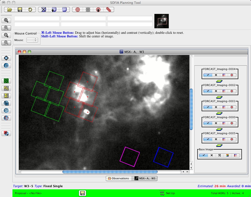
We point out first, it is likely that given the small overlap of these fields the problem of not fully sampling the area will occur at certain field orientations. Additionally however, let's assume that the GI needs 10 minutes per position to integrate down to the level required of the science. Let's also assume that for this source, the sky is rotating rapidly enough that the telescope needs to perform an LOS rewind after every 10 minutes. In that case there would be an LOS rewind after each element is sampled in the mosaic. Assuming that this rotation is the maximum 3 degrees, the final sampling of the field will look more like this:
In the above example where each field has rotated an additional 3 degrees from the last one, the final field (upper left red box) has rotated a total of 12 degrees different from the first field of the mosaic (lower right red box). This again demonstrates why it is important for the GI to make sure that their mosaic fields will overlap enough that field rotation will not be a problem.
2.4. Dithering an Imaging Observation
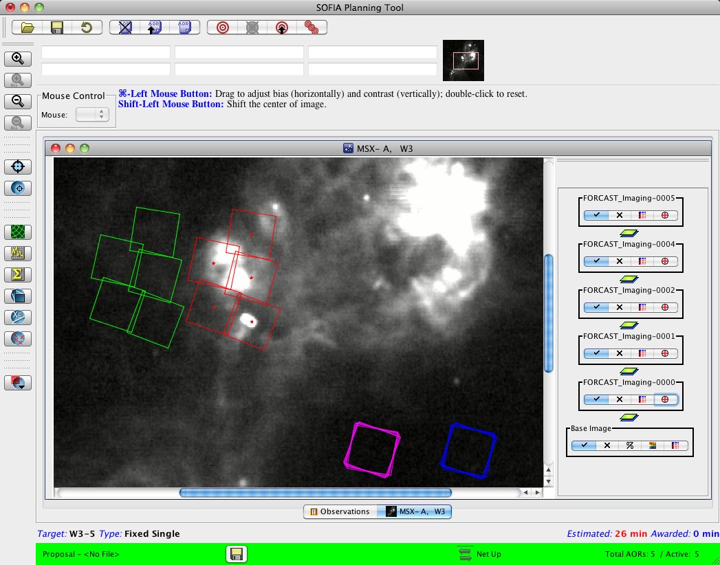
The FORCAST array is relatively clean cosmetically for most observations. For very bright extended sources, there can be some array artifacts present. Removal of some of these effects can be accomplished with dithering. Dithering refers to small movements (of the order of 10-15") of the telescope which place the imaged object at different locations on the array. Typically one dithers 3 or 5 times. Shifting and then median combining these images can remove any patterns that are positionally dependent on the array. For faint sources (those not immediately detectable in a few minutes), it is best if no dithering is performed (because the shifting and adding of dithers cannot as yet be performed reliably for fields without brIf you are imaging a bright and extended source and wish to dither, both C2N modes can be performed with dithers included. GIs should be aware, however, that dithering results in additional overheads that can be significant for short observations or observations with a large number of dither positions (see the example in the last paragraph of Section 2.2.1 ). These additional overheads are included in SSpot observation time estimates. Instructions for how to set up dithers is straight forward and given in the SSpot Handbook. An example of what a 5-element dither with 10" offsets looks like can be seen below. Here the field of interest ("NodA-Chop1") with the 4 dither offsets are being visualized without the reference fields to show the dither offsets more clearly.
3.1. Setting up the Acquisition Image The first step in designing a spectroscopic observation is to set up the initial acquisition images. To do this, the user selects "FORCAST Acquisition" under the "Observation" menu. This generates a new aquisition AOR, the main panel for which is shown below.
Since it is important for the acquisition image configuration to be the same as that of the science observations, one can select an AOR that has the appropriate configuration and import that into the acquisition AOR. This is done by selecting the desired AOR template from the "Import Config from AORID" dropdown menu. The Order number of the AOR should be one less than that first grism observation. The GI only needs to make one set of acquisition AORs per target per slit used. The recommended filters to use for each grism are as follows: F077 for G063 or XG063; F111 for G111 or XG111; F197 for G227; and F315 for G329. If you believe it to be necessary, other filters may be used for acquisition only after discussion with your Support Scientist. The GI should then estimate the integration time necessary to achieve a S/N ≥ 5 in that filter. It is assumed that for most spectroscopic targets, this will be on the order of 10-60 seconds. Every acquisition will add 5 minutes of duration to your program.
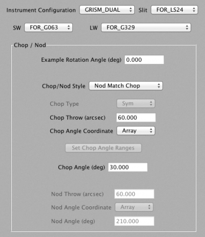
3.2. Setting the Instrument Parameters for Spectroscopic Observations The basic layout of the main AOR panel for grism observations is the same as that shown above for imaging observations. The main difference is in the instrument configuration portion of the window as shown below.
The desired on-source integration time should be determined by using the FORCAST Grism Observation Calculator and is entered into the "Exposure Time" field. This value does not include overheads. In some cases, GIs may wish to dither their observations. In this case, there are two possible approaches to conducting the observations - one can step through each position in the dither pattern once until the pattern is complete, or the dither pattern can be looped through multiple times until the total on-source time is achieved. In general, it is better to only loop through the dither pattern once as this minimizes the overheads associated with the observation (and maximizes the observing efficiency). In some cases, however, GIs may desire to loop through the dither pattern. This can be specified with the "Cycles" field. The total on-source time will be the value entered into the "Exposure Time" field multiplied by the number of "Cycles". Note that at this time, SSpot does not properly account for the additional overheads associated with looping through a dither pattern. GIs who wish to pursue this option should discuss it with their Support Scientist. In some cases, it is necessary to split an observation among multiple flight legs. The "Min Contiguous Exp Time" field should be used to provide flight planners with information on the minimum amount of time that can be scheduled for a single flight leg to be scientifically useful. For example, if a program has been awarded 2 hours of time for imaging a faint target, it may be necessary to divide the observation over multiple flight legs. If the source is faint enough to require at least 15 minutes on-source in order to be able to accurately coadd the data from multiple flight legs, then this should be entered into the "Min Contiguous Exp Time" field. " When pipeline processing FORCAST spectroscopic data, it is useful to know whether or not the source is extended or point-like in the IR. Setting the "IR Source Type" ensures that the proper extraction routines are used during processing of the science data. Finally, the GI must select the appropriate instrument configuration, grism, and slit for the AOR. The options in the "Instrument Configuration" panel include both single channel modes (GRISM_SWC and GRISM_LWC) and dual channel mode. Note, however, that even though users are allowed to select GRISM_DUAL, dual channel grism mode will not be allowed for Cycle 4.
3.3. Setting the Chop/Nod Parameters for Spectroscopic Observations
As is the case for imaging mode, the majority of spectroscopic observations with FORCAST will involve objects that are relatively compact (source diameters <120") and lie in areas of the sky free from contaminating extended emission. For such observations, using the Nod-Match-Chop (NMC) chop/nod mode is recommended. Because coma will increase with larger chop throw (1" of coma for every 60" of chop throw in NMC mode), the GI should configure chop throws to be as small as possible, but large enough that they know they will be chopping off of their source and onto clean sky. If there are clear chop reference areas all around the science source, it is recommended that the NMC mode be used and configured with a chop angle of 30 degrees and in the "Array" chop angle coordinate system for long-slit spectroscopic mode.
If the source is surrounded by or has nearby extended emission, the GI will have to configure the chop throw and angle in the "Sky" chop angle coordinate system to avoid contamination in the chop reference fields. This is discussed in more detail and with examples below . This is also where you will find a discussion of using the NXCAC mode for performing spectroscopy on very large extended objects. NXCAC (Nod Unrelated to Chop/Asymmetric Chop) mode is analogous to C2NC2 mode for imaging in that it is less efficient but allows for large throws without negatively affecting image quality.
The GI also may or may not wish to dither the observations along the slit. There is a section below that discusses the general rules of thumb for using dithers with FORCAST.
We do offer a Nod-Perpendicular-to-Chop (NPC) mode as well in SSpot for the long-slit spectroscopy only (this mode is not available for cross-dispersed spectroscopy). If you are an experienced IR observer and have a good reason why you wish to use this mode instead, please discuss this with your SOFIA Support Scientist. The GI may choose between two special NPC setups: Nodding Along the Slit (NAS) or Chopping Along the Slit (CAS). As is the case with imaging mode, and contrary to popular belief, there is no sensitivity advantage in using one of these NPC modes over NMC mode, as both modes yield the same S/N in the same exposure time (as discussed here and here ).
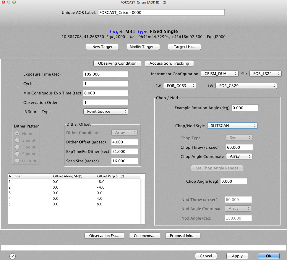
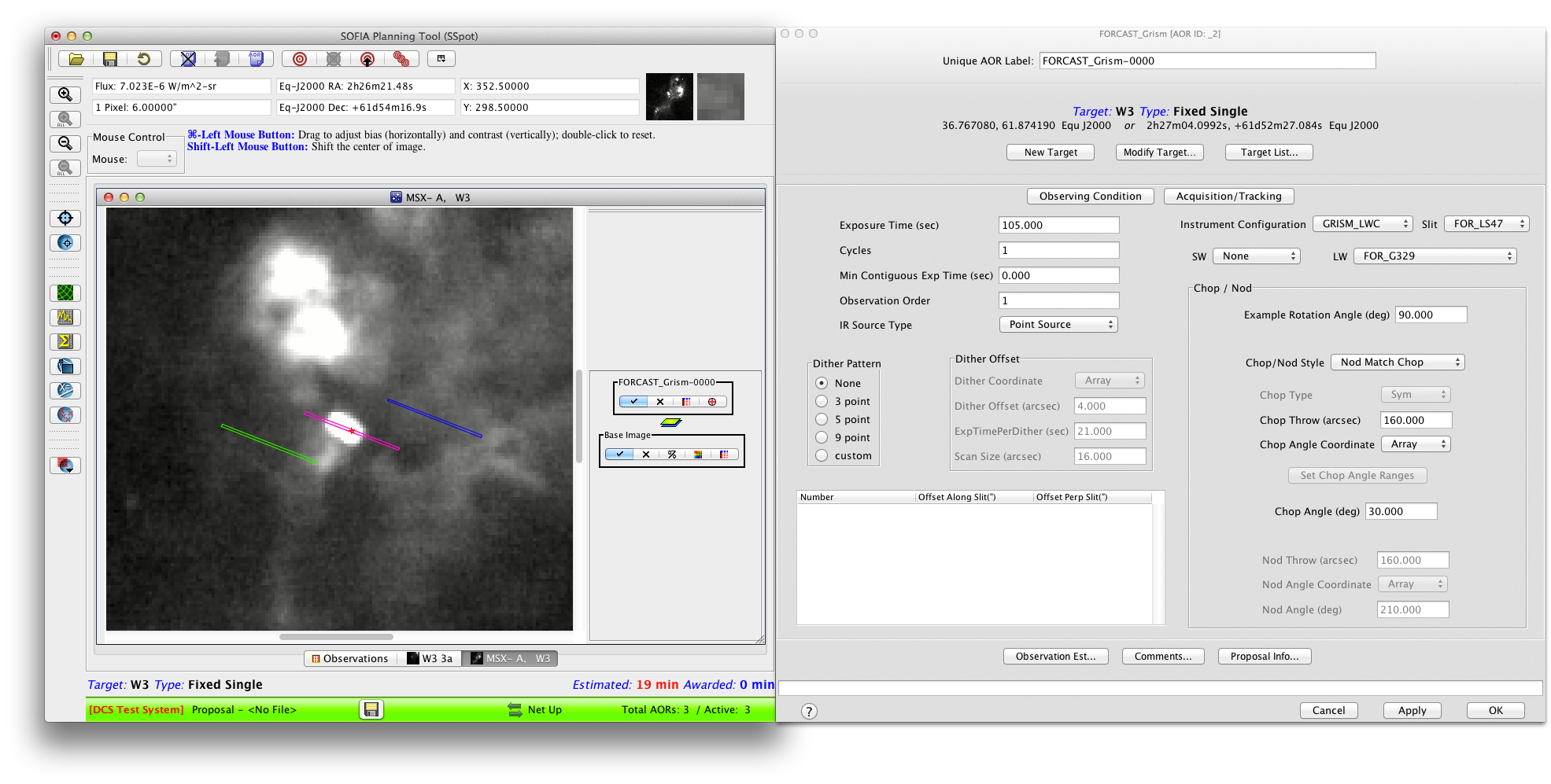
It is also possible to perform slit scan observations of extended sources with FORCAST grisms, wherein spectra are acquired at a number of positions across the source as defined by the GI. Selection of "slitscan" mode is by the Chop/Nod Style drop-down menu in the Chop/Nod section of the AOR definition box (see below). This mode is defined by specifying a set of dithers that offset the telescope perpendicular to the slit. Once "slitscan" mode has been chosen, the default five position dither pattern is loaded into the dither panel. The default scan pattern is defined with the spacing between each consecutive slit position equal and with the scan pattern centered on the given source position. So, for example, if the GI wants the slit scan to include 5 slit positions with overlapping coverage, then they might set the dither pattern as shown below. Since the wide long slit is 4.7'' wide, setting a dither offset of 4'' will result in a slit overlap between consecutive slit positions. The GI does not explicitly set the number of positions in the scan. Instead, the number of discrete slit positions is determined by the user specified Dither Offset and Scan Size, i.e. the total length of the scan. The number of slit positions, then, is the scan size divided by the dither offset, rounded up, plus 1. Since the slit scan is performed perpendicular to the slit, this mode can only be performed in array coordinates. This means that the actual orientation of the scan on the sky will not be known until after flight planning.
3.5. Dealing with Extended Objects and/or Complicated Environments
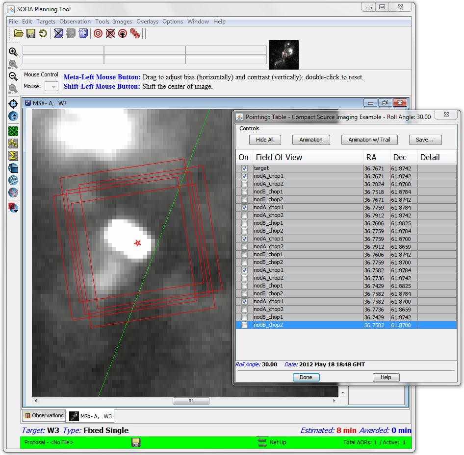
In the example below, a long-slit spectroscopic observation using a NMC set up is shown on the bright elongated object at the center of W3. The long red rectangle shows the long slit centered on the source to be observed, while the long green rectangle and long blue rectangle show the chop/nod reference slit positions. This chop/nod set-up is configured in "Sky" coordinates so that the chop/nod reference positions avoid the bright nearby emission to the north of this science target. However, as can be seen in the example below, there still appears to be extended diffuse emission contained in the reference slit positions (as seen in the MSX image). If the observations are short, the extended diffuse emission contained in the reference slit positions may not be a problem. The GI must confirm that this emission is below FORCAST's detection level given the exposure time of the proposed observations and the wavelength dependence of the extended emission. However, if the GI wishes to perform deep observations of the region or is unsure if the extended emission in the reference fields will be a problem at the particular wavelengths to be observed, then s/he should try to chop and nod farther away. However, beyond about 180", the chopped sources will have significant coma (>3"). Though image quality is less of an issue for spectroscopy than imaging, a large coma will decrease the effective brightness of the source by spreading out the flux, thus decreasing the expected S/N of a spectrum in a given amount of exposure time. If very large throws are needed to reach clean sky, the GI should configure the observations using NXCAC mode. Please note that these observations are much less efficient (about 3.5 times longer duration than C2N modes), so if you were awarded time for your observations under the assumption that NMC or NPC mode would be used but you find during Phase II that you will require NXCAC, you will have to observe with fewer grisms or observe fewer targets to still fit the NXCAC observations within the awarded time.
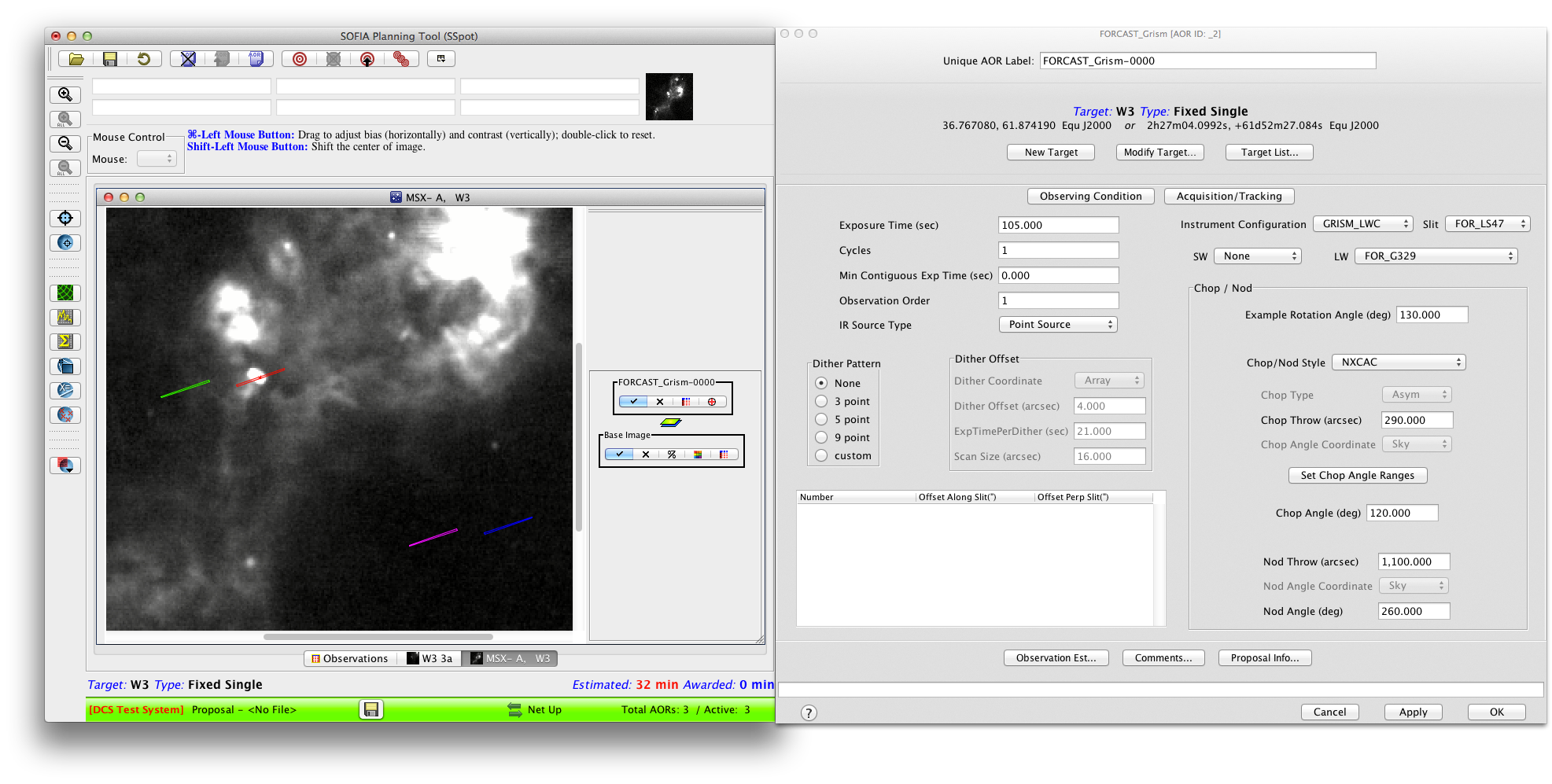
Below is a spectroscopic setup in NXCAC mode , which allows chop throws up to 8 arcminutes and nod throws up to 10 degrees. In this asymmetric chop mode sources will have no coma and one can sample clean sky relatively far from sources. If the GI wishes to perform very deep spectroscopic observations on the source of interest (long red rectangle), s/he can configure the chop to be far away and at an angle that will get the chop reference slit positions on much cleaner sky (long green rectangle). The nod position is then chosen to be far enough away that there is no chance of environmental emission in those slit positions (long blue rectangle and long purple rectangle).
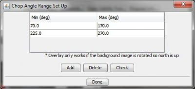
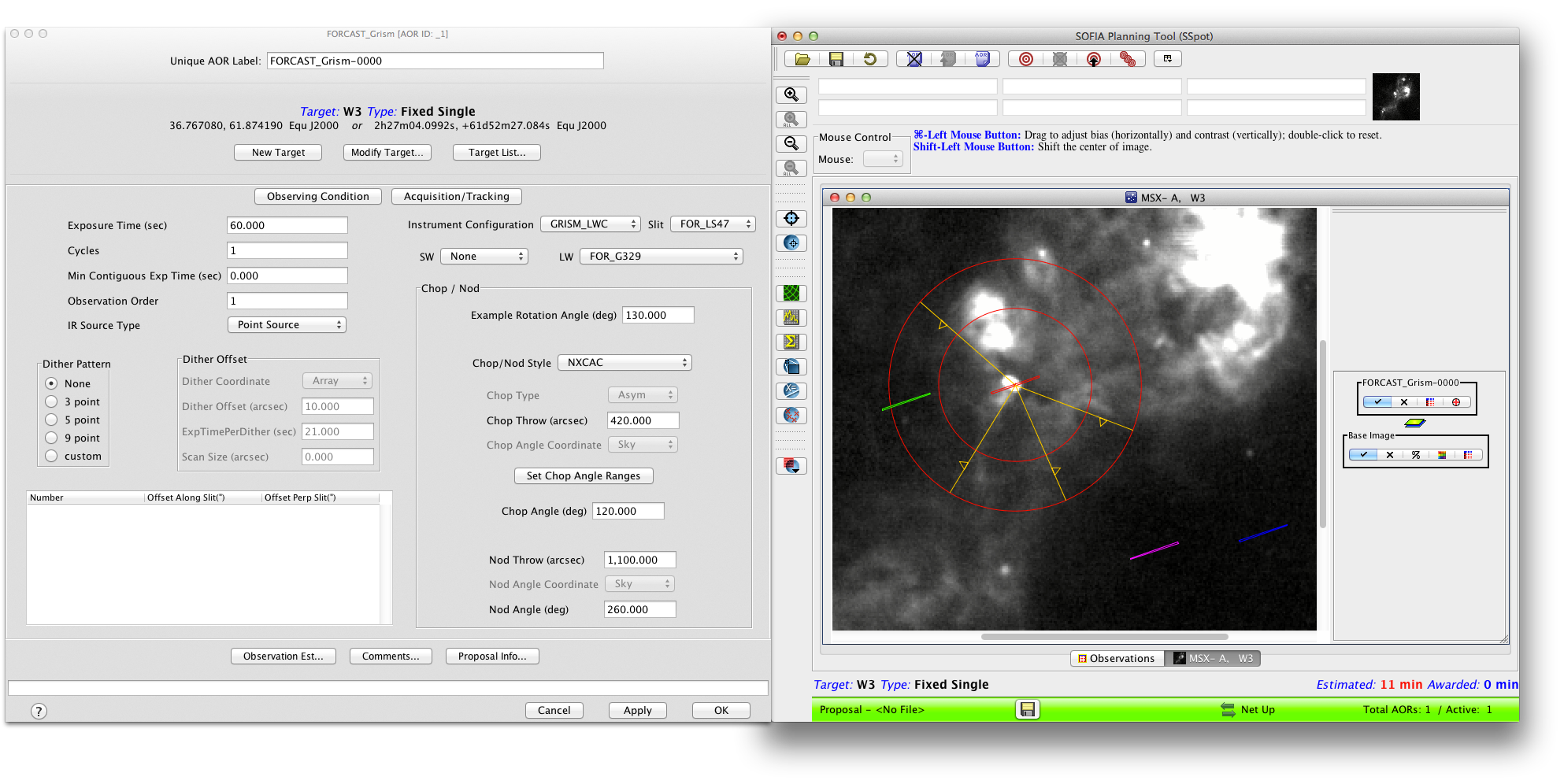
The above set-up will work up to a chop thow of 250". If chops larger than this are still necessary to reach a chop reference field of fainter background emission, then the NXCAC AOR setup must be configured with a preferred chop angle and a range of other possible chop angles in the likelihood that the preferred angle cannot be used (due to hardware limits involving the sky rotation angle at the time of observation). Below is an example of this setup for W3. The preferred chop angle of 120 degrees is shown as the long green rectangle, and two alternate ranges are shown: one from 70-170 degrees, and the other from 225-270 degrees (as specifiied in the "Chop Angle Range Set Up" diaglog window), and shown as the orange-to-cyan lines. Notice these angles encompass the cleanest sky areas in the MSX image for this region, and thus are likely to be suitable for chop reference slit positions for very long integrations. At the time of observing, a chop angle will be chosen from these ranges if the preferred angle is not possible. It is in the GI's best interest to specify as large a range (or ranges) of chop angles as possible.
3.6. Dithering a Spectroscopic Observation
The FORCAST array is relatively clean cosmetically for most observations. For spectroscopic observations, a spectrum may lie across a bad (or hot) pixel(s) and could be misinterpreted in the extracted spectrum as a line. To mitigate this, we set up our calibration stars on the same pixel as the science targets, which means that the science spectra are dispersed over the same pixels of the array as the calibration spectra. Any pixel-to-pixel variation should therefore be removed when the science data are divided by the calibration data. For extended sources, the removal of such cosmetic issues can be accomplished with dithering. Dithering refers to small movements (of the order of 3-15") of the telescope which place the imaged object at different locations along the slit and, therefore, place the spectra at different positions on the array. In spectroscopy, typically one dithers 3 or 5 times along the slit direction only. Shifting and then median combining these images can remove any patterns that are positionally dependent on the array. For faint sources (those not immediately detectable in a few minutes), it is best if no dithering is performed. If you are imaging a bright source and wish to dither, any of the spectroscopic observation modes discussed (NMC or NXCAC) can be performed with dithers along the slit included. Instructions for how to set up dithers is straight forward and given in the SPPOT Handbook. GIs who have a strong justification for dithering in this mode should discuss this with their Support Scientist.
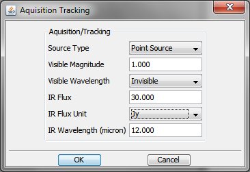
4.1. Specifying Visual Magnitude of Target
It is important to check the visual magnitude of each science target. If the target is brighter than 14th magnitude and point-like (i.e., compact), then the GI should give the magnitude and the reference wavelength (band V, B or R) in the "Aquisition Tracking" pop-up window (see below). In this case, the telescope can guide on the source directly, which greatly decreases observation set-up overhead and translates to more time taking science data on the target during a scheduled flight leg. If the object is fainter than this, the GI should select "Invisible" from the "Visible Wavelength" pull-down (any value in the "Visible Magnitude" field will then be ignored).
It is also a good idea to fill in the IR flux of the source at a reference wavlength close to the one being observed. This helps the observer to assess whether or not the observations are proceeding as expected.
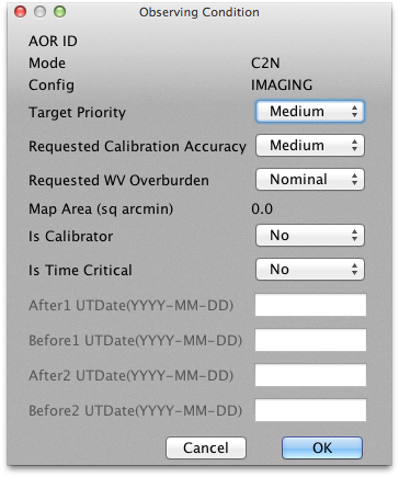
4.2. Setting Priority Between Targets in Your Program
In the "Observing Condition" pop-up window (see figure below), there are two keywords that help a GI prioritize their observations. The pull-down menu for "Observing Priority" refers to the relative priority of a specific science target with respect to other science targets within the GI observing program. This is used by the flight planners to determine which observations to schedule if for some reason not all of the targets within the GI's program can be observed. The GI can select a target to be either Low, Medium, or High priority. If all of the GIs targets are of equal interest (as for, say, a survey of many dozens of targets), then they should all be set to Medium (the default). Setting all of the targets to High priority will not ensure that they all are observed. If High priority is used for some targets, other targets must be set to Medium and/or Low priority as well.
4.3. Setting Priority Between Observations of a Single Target
The most important parameter to set in terms of observation prioritization is given by the "Order" parameter. This field allows the GI to numerically list the priority of their observations of a single target within an observing leg. The length of an observing leg is rigidly defined during flight planning and cannot be extended in flight. If, for instance, acquisition takes an unusually long time, or if there are any hardware/software failures during the observing leg for a particular target, it may be that not enough time will remain for all of the scheduled observations of the target to be performed. For this reason we ask the GI to prioritize their observations. If achieving the full exposure time in some filters (or grisms) over others is most important to a program, then we request that the GI order their filters serially, i.e. the first observation to be executed will be Order=1, the second will be Order=2, and so on. In this way, if time is cut short on an observing leg, the GI will get all of the time in the observations with the lowest Order values, but may get little or no time for the observations with the highest Order values. However, if the GI thinks that it is better to get some time in all filters/grisms, and that if any time is lost it is taken from all observations equally, then the GI should break up the observations of a single AOR into multiple smaller AORs and prioritize them using the Order parameter so that we will be essentially looping through all filters throughout the leg. Here is a simple example that shows how breaking up AORs of a single target would be advantageous. A GI wants to observe Jupiter for 40m with 20m in the 37.1 μm filter and 20m in the 7.7 μm filter. If the GI gave the 37.1 μm filter Order=1 and the 7.7 μm filter Order=3, and a 40m leg is scheduled but an in-flight computer malfunction leads to a loss of 20m on the leg, then the GI will end up with a 20m observation of Jupiter in the 37.1 μm filter, but no 7.7 μm observation. If, instead, the GI split each 20m AOR into two 10m AORs and gave the first 37.1 μm filter Order=1, the first 7.7 μm filter Order=2, the second 37.1 μm filter Order=3, and the second 7.7 μm filter Order=4, this would have the effect of looping twice through the filters with half the time in each visit. Therefore, during a 40m leg with a 20m time loss, the GI would end up with about 10m in both filters (or ~70% the S/N of 20m observations; however note that there is also some small additional loss of efficiency due to filters changes).
4.4. Setting Calibration Accuracy
The GI may be worried about the calibration accuracy of their observations. The "Required Calibration Accuracy" is a pull-down menu that allows the GI to let us know if accurate calibration is important to their program. For Cycle 1, we expect to deliver flux calibration at the level of 20% absolute accuracy, and while we expect to do better than that in many cases, we can make no guarantees to do better than that for a particular observation. However, there are times in flight (i.e. after the first 2 hours) where calibration is usually better. If the GI sets the "Required Calibration Accuracy" to High, the flight planners will make a best effort to put these observations in the flight plan at times when we usually have better calibration accuracy (but again, for Cycle 1, we cannot guarantee better than 20% accuracy, regardless of what is requested for the Required Calibration Accuracy).
The GI may also be concerned about needing extra sensitivity for a particularly challenging observation. Generally, the higher the aircraft flies, the smaller the water vapor overburden and the greater the sensitivity of FORCAST (especially at wavelengths >25 microns). If a GI has a particularly faint target, s/he may wish to change the "Required WV Overburden" from Nominal, to Low or Very Low. However, like the calibration accuracy pull-down menu, in Cycle 3 we cannot guarantee that the observations will be taken under low water vapor conditions. Again, however, the flight planner will make a best effort to accommodate such requests by scheduling the observations at the highest altitudes.
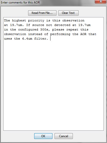
4.6. Including Instructions to the Observers/Planners
It is very likely that most or all of the GI's observations will be performed without them onboard the aircraft. Therefore it is vitally important that the GI convey any special requests or procedures to the observer through the comment tool. These comments will be read by the observers in flight. They will also be viewed by flight planners. Therefore any comments to either one of these groups should be written in the text field of this pop-up window (see example below). These comments will be reviewed by your Support Scientist during the Phase 2 process to ensure that they are thorough, clear, and understood.