This module is the first executable module of SPICE extraction flow, and it must be executed prior to the Ridge module. It will compute and plot the mean spatial flux profile across all user-selected orders in the same slit. The wavsamp.tbl calibration file is used to specify the location of the selected orders.
INPUTS
(High or Low) Res Order: SPICE will assign default orders to be used in measuring the spatial profile. The module input will be labeled either High Res Order or Low Res Order depending upon the information in the BCD FITS header. In High Res (channels 1 and 3), all orders (11 - 20) are used by default. In Low Res (channels 0 and 2), the default order depends upon the commanded field of view (e.g. an observation in LL-2 will default to orders 2 & 3). Alternately, the orders to be used by Profile may be chosen by the user from the pulldown menu (in High Res, use the Select Orders option in the pulldown menu to activate the checkbox list of orders. The checkbox list can be accessed via the right-hand arrow).
OUTPUTS
Profile Output Table (*.profile.tbl): The output of Profile is a table of the wavelength-collapsed average spatial profile for the selected orders in the same slit. It can be viewed as an ASCII table by clicking the View button. The graph of flux vs. spatial position (percent across the detector from x = 0) is shown in the plot window.
DISCUSSION
This module computes a wavelength-collapsed average spatial profile of all orders in the cross-dispersed IRS image. It takes the mean of all orders at a given spatial position and produces a table of the average flux distribution and the corresponding standard deviation for each of N positions across the orders. It uses the wavsamp.tbl file to specify the location of the orders.
The Profile module takes as input the two-dimensional Level 1 Basic Calibrated Data (BCD) dispersed image in FITS format. This module does not consider the pixel status mask associated with the BCD file. The module averages the spatial profile over all selected spectral orders. By default, all orders are used.
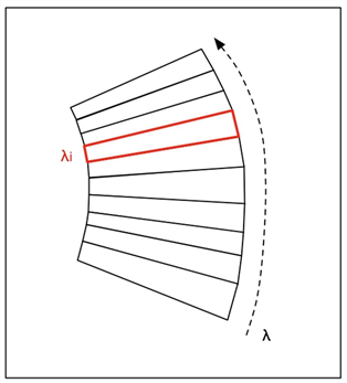
The input wavsamp.tbl file specifies the location of the spectral orders on the array in x-y coordinates. It consists of "pseudo-rectangles" which describe the fractional pixels that comprise each wavelength in the spectrum (see Figure 2.3.1). These pseudo-rectangles are specified by their four vertices. Each line of the wavsamp.tbl file consists of an order number, coordinates of the center of the pseudo-rectangle (x center, y center), wavelength, tilt angle, and four vertices (x0, y0, x1, y1, x2, y2, x3, y3). Table 2.3.1 shows an example of the wavsamp.tbl.
Table 2.3.1: Sample wavsamp.tbl file.
\wavsamp version 5.0 (Thu May 9 10:19:35 PDT 2002)
\processing time 17:05:26 PST 03/12/2003
\comment WAVSAMP SL, generated from b0_ordfind.tbl 03/12/03
The Profile module divides each pseudorectangle in each order into N_CUTS parts and integrates the signal within each part (100 parts in the lights-out pipeline; 1000 parts in SPICE). The integral is divided by the area of each part to yield the average signal at that wavelength. A running sum is kept as this procedure is repeated for each wavelength in each of the orders to be considered. The standard deviations are calculated from the signal and the square of the signal.
NOTE: The profile is calculated as a function of left-to-right percentage along the spatial direction of the slit.
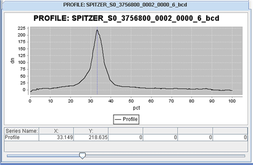
The output of Profile is a table describing the average signal and sigma in each of the N_CUTS sub-rectangles. The default name of this file is profile.tbl. Figure 2.3.2 shows an example of the profile calculated from a SL observation of a faint source on a complex background. An excerpt from a profile.tbl table for the same module is shown in Table 2.3.2.
Table 2.3.2: Sample profile.tbl file (excerpt).
\int CHNLNUM = 0
\int FOVID = 27
\int ORDER1 = 1
| pct | dn | stdev | n | region |
| real | real | real | int | int |
0.50 2.5838E+01 4.1910E+01 108 0
1.50 3.1066E+01 4.0129E+01 108 0
2.50 3.0284E+01 3.7313E+01 109 0
3.50 2.8732E+01 2.2572E+01 113 0
4.50 2.8311E+01 2.0112E+01 121 0
5.50 2.6560E+01 1.8742E+01 129 0
Figure 2.3.1: One spectral order defined by the wavsamp.tbl file is illustrated, with a single pseudo-rectangle highlighted. Order curvature is highly exaggerated here for illustration.
Figure 2.3.2: An example of the outputof the PROFILE module.