For each flow, SPICE allows visualization of both the input images and the output spectra. Two-dimensional images are displayed in the FITS window, and one-dimensional spectra and plots in the Plot window. The current display in either window can be saved.
1.7.1 FITS Window
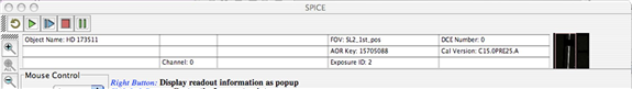
The FITS window (Figure 1.7.1) displays the input BCD images, which are the two-dimensional spectra. The controls at the left of the SPICE window allow the user to zoom in and out. The �Base Image� panel in the FITS window allows the user to control the opacity of the image, change the stretch and color table, and view the FITS header. The entire panel containing the �Base Image� options and all other overlays can be moved with respect to the FITS image itself by clicking on the textured edge of it and dragging. This panel can be dragged within the same FITS Window, or it can be dragged outside of it (click on the red X to return it to the window). A few header keywords (Object Name, Channel number, AORKEY, FOV, CalSet) are displayed at the top of the SPICE window when the cursor is in the FITS display (see Figure 1.7.2).
Figure 1.7.1: The FITS window, displaying the BCD data file with the spectral trace.
1.7.1.1 Pixel Values
SPICE also displays pixel information at the top of the window as the cursor is moved within the display. This information includes the RA and Dec corresponding to the sky position of that pixel; recall that the spatial direction is approximately parallel to the x-axis in the image. The pixel information also includes the approximate wavelength (microns) at that pixel, and it's approximate spatial offset from the slit center (arcsec). The pixel information can also be accessed by right-clicking the mouse at the pixel of interest to bring up a popup window. Only one such window can be accessed at one time.
Note that the RA and Dec displayed in channel 0 (short-low) can refer either to the position within the slit or the position on the PeakUp array. The coordinates within Red and Blue Peak Up are approximately contiguous on the detector. But they are not contiguous with the RA and Dec within the spectral slits.
Figure 1.7.2: The BCD and pixel information window
1.7.1.2 Overlays
SPICE will overlay the ridge line and extraction windows on top of this image when they are defined by the corresponding modules. These overlays may be toggled on and off, and their colors may be changed.
1.7.1.3 Saving the Image
The image and overlays displayed in the FITS window can be saved in a variety of formats from the File menu.
1.7.2 New FITS windows
Users may find additional FITS display windows useful for examining serendipitous sources within the slit. Additional FITS display windows can be opened in two ways: from the Initialize Parameters and Files module once it has been run (choose a Reference Image from the drop-down menu and click on View), and from the Images menu in the main SPICE toolbar. The controls to the left of the SPICE window allow the user to perform a variety of image functions, such as zooming in and out, re-centering, and computing the distance between two points. The opacity, stretch, and color table can be modified within the Base Image section of the FITS window. This section also allows the user to display the FITS header. The entire panel containing the Base Image options and all other overlays can be moved with respect to the FITS image itself by clicking on the textured edge of it and dragging. This panel can be dragged within the same FITS Window, or it can be dragged outside of it (click on the red X to return it to the window). If the FITS display window is opened from the Initialize Parameters and Files module, it will show the IRS slits. If, in addition, the ridge is set manually, the ridge position will be shown within the IRS slit.
1.7.3 Plot Window
The plot window displays the results of each module (see Figure 1.7.3). It allows interactive changes to the plot ranges. To change the plot range, hold down the Left-mouse button and drag the mouse to select the range to be displayed. The box must be dragged from the Upper-Left corner to the Lower-Right corner. Dragging up-and-left will return to the original range.
A number of options are available in a drop menu by holding down the Right-mouse button over the plot:
Properties: Selection of the plot titles, ranges, and color.
Save as....: Save the plot as a .PNG image.
Print...: Send the plot to the printer.
Zoom In/Out: Zoom one or both of the axes in or out. The "Domain" axis is the X-axis. The "Range" axis is the Y-axis.
Auto Range: Return to the original axis ranges.
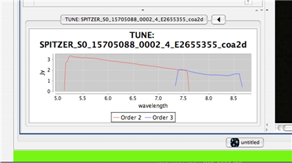
The window includes the option to display the results for Profile, Extract and Tune. The choice is made using the arrow (or tab, depending on your operating system) at the top of the plot window. The plotted spectra are color coded by order. The Profile display allows interactive selection of the Manual Ridge percentage, using the slider at the bottom of the tab.
Figure 1.7.3: The Plot Window, showing the results of the Point Source Tune module. The displayed output can be changed using the arrow button at the top of the window.